Circuits and Systems
Vol.3 No.3(2012), Article ID:20196,5 pages DOI:10.4236/cs.2012.33028
Reactive Compensator Synthesis in Time-Domain as an Alternative to Harmonic Method
Electrical and Computer Engineering, Cracow University of Technology, Kraków, Poland
Email: e-3@pk.edu.pl
Received July 6, 2011; revised March 1, 2012; accepted March 8, 2012
Keywords: Power and Energy Theory; Reactive Power Filters; Reactive Current; Optimization; Harmonic Filter Design
ABSTRACT
The source reactive-current compensation is crucial in energy transmission efficiency. The compensator design in frequency-domain was already widely discussed and examined. This paper presents results of a study on how to design reactive compensators in time-domain. It’s the first time the reactive compensator has been designed in time domain. The example of compensator design was presented.
1. Introduction
This article is a discussion on issue raised in the article of L. S. Czarnecki [1] where the author consider if it is possible to make current decomposition into active, reactive and unbalanced current in time domain and basing on it build reactive compensators. The current decomposition in time domain was presented in the previous articles [2, 3] and in this article is presented the reactive compensators design in time-domain.
2. Reactive Current Compensation in Time-Domain
In the article [3] was shown that source-receiver current can be decomposed into active and reactive current in “s” domain i.e. for Laplace transform of signals. Reactive current can be compensated with the reactive compensator. The source-receiver current decomposition is given below:
 (1)
(1)
where:
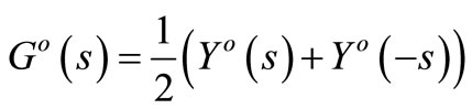 (2)
(2)
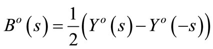 (3)
(3)
stand for the active and reactive parts of receiver admittance operator Yo(s).
The I(s) transform for T-periodic signals is derived using the following relation between non-periodic and periodic signals transform [3].
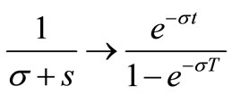
 (4)
(4)
where t Î [0, T), Re(σ) > 0, T-time period.
It can be also calculated directly in time-domain as the T-periodic convolution:
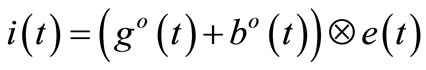 (5)
(5)
where go(t), bo(t) stands for T-periodic impulse response of admittance active and reactive part.
Connecting in parallel the compensator (Figure 1) the reactive current balance in time-domain states that:
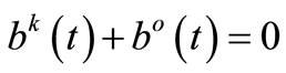 (6)
(6)
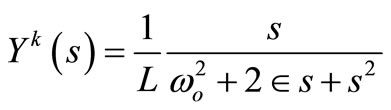
3. T-Periodic Impulse Response of Compensator and Receiver
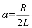
Admittance of the elementary RLC compensator branch
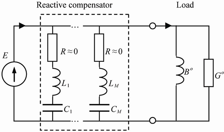
Figure 1. The zero impedance source with receiver and almost lossless compensator connected in parallel.
is:
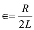
 ;
; ;
; 
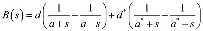
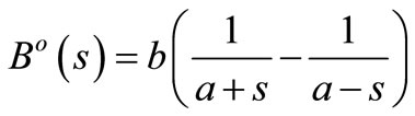
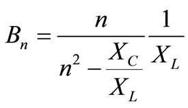
(We assume later that the compensator is composed of almost lossless elementary branches). And its reactive part is then (3)
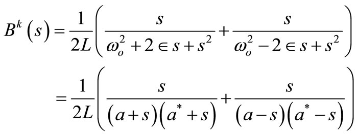
which leads to general form
 (7)
(7)
where L(s), M(s)—odd and even polynomials.
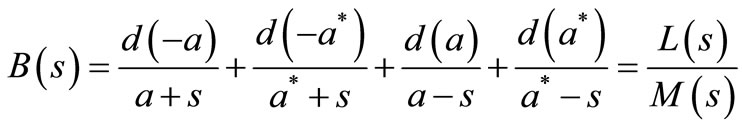
The residues meet the relations: if
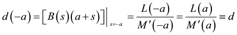
then:
 ;
; ;
; 
where:
M′(s) is the derivative of M(s) with respect to s, d— real number.
Thus (7) reduces to
 (8)
(8)
and under (4) and trigonometric identity


where aT = α + jβ.
We get
 (9)
(9)
In the case of almost lossless compensator i.e. for α → 0.
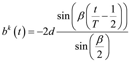
 (10)
(10)
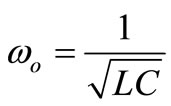
where:
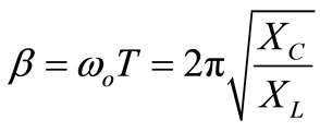
 ,
, —capacitive and inductive reactance for the main frequency
 .
.
Residue for Bk(s) in  can be calculated as
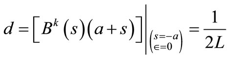
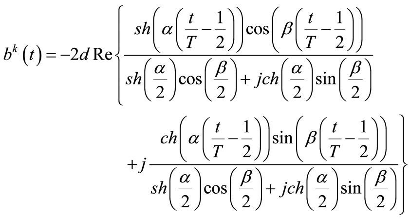
Thus the T-periodic impulse response of reactive part of the elementary RLC branch (without R) has form
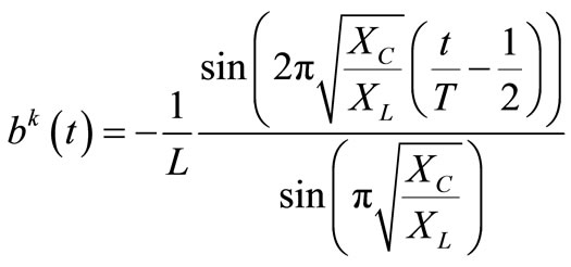
 (11)
(11)
where:
 ,
,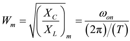 —angular and relative resonance frequency of m-th branch, and is depicted in Figure 2.
Later, in the article, it assumes that the reactive part of receiver Yo(s) has only real poles, so the receiver is nonoscillatory circuit not as the compensator.
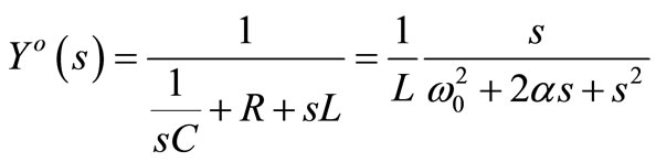
For the single pole receiver e.g. RL or RC type the operational admittance is

thus its impulse response is
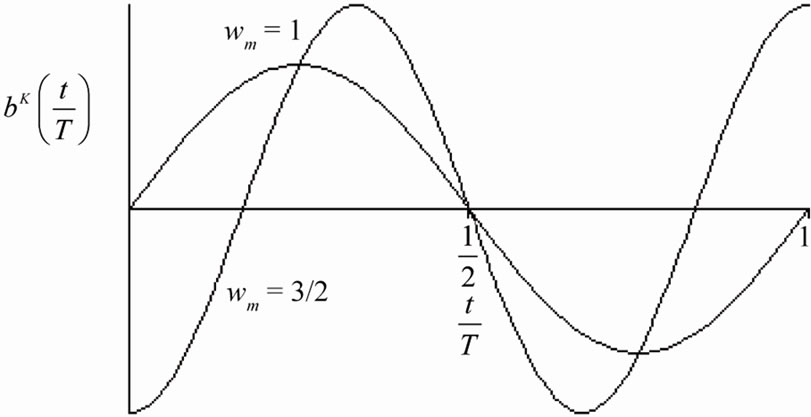
Figure 2. T-periodic impulse response of the compensator elementary branch.
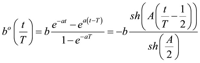 (12)
(12)
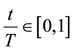
where A = aT,  Î [0, 1).
The coefficient b can be both positive and negative what is shown below for the RRLC receiver (see Figure 3).
Its operator admittance is
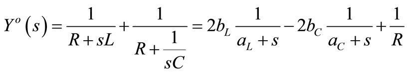
where ,
,  ,
,  ,
, 
Then the reactive part of Yo(s) is
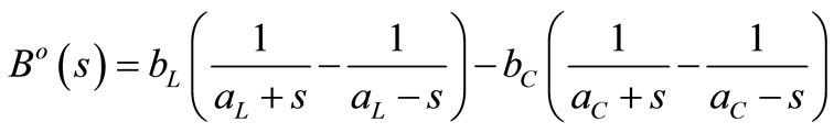
and its T-periodic impulse response is
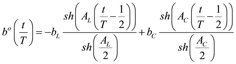
where AL = aLT, AC = aCT.
For the receiver shown in Figure 4, the operational admittance is
where ,
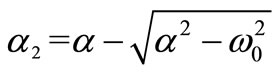
,  and for the positive poles
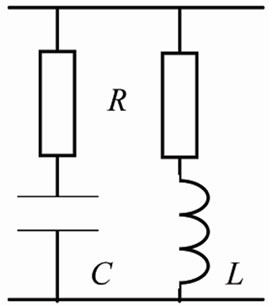
Figure 3. Example of the RRLC load.
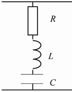
Figure 4. Example of the RRLC load.
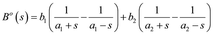
 , Yo(s) takes form
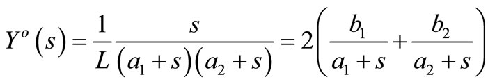
where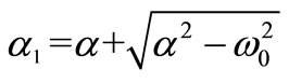 ,
,  and the coefficients b1, b2 are then
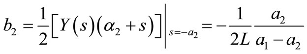

thus
The reactive function  (12) is shown in Figure 5. It is necessary to distinguish the two cases when b > 0 and b < 0. When
  → 0 the curve become straight line.
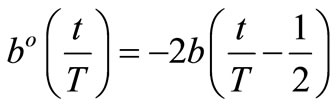
 (13)
(13)
because sh(x) → 0 for x→ 0.
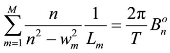
Thus we arrive to the compensatory balance Equation (6) in a new form
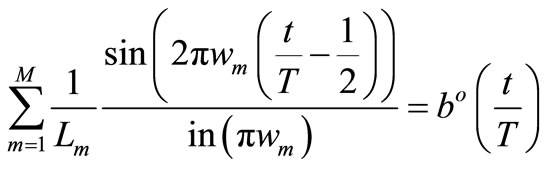 (14)
(14)
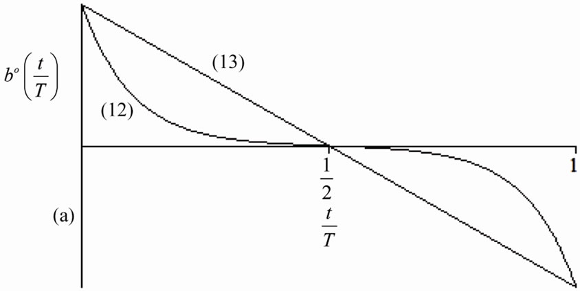
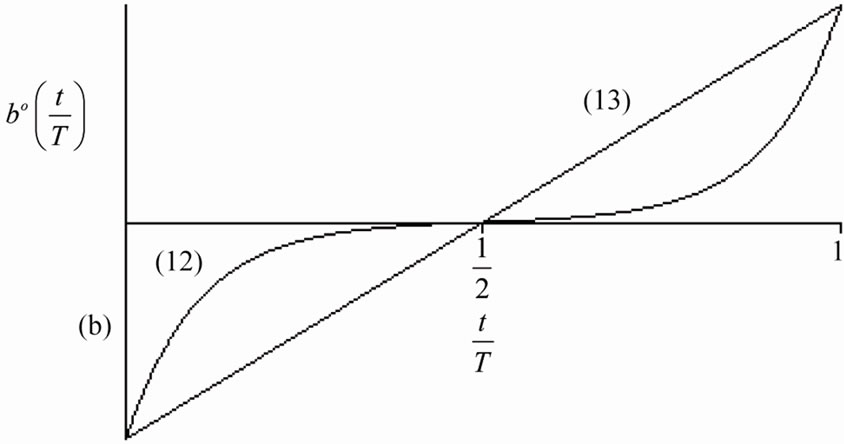
Figure 5. T-periodic single pole reactive operator impulse response of the load (a) RL (b > 0); (b) RC (b < 0).
where M—total number of compensator branches.
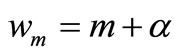
The solution of (14) (see Figures 6 and 7) for the unknowns Lm and Cm, can by find with optimization method. The (14) can be rewritten in respect to Dm and wm
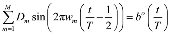 (15)
(15)
where
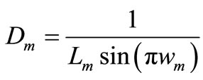 ,
, 
The relative frequencies of LC compensator branches have to meet the condition
Thus we must choose relative resonance frequency wm of compensator branches as not the even numbers  ; p—even number.
The set of Equations (14) can be then solved for Dm by minimizing .
.
 (16)
(16)
where
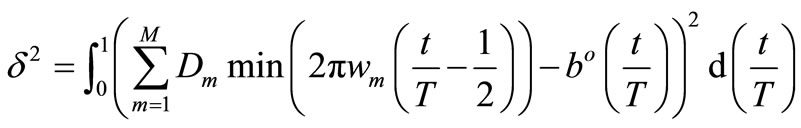
After equate to zero appropriate partial derivatives
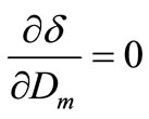
and assuming that
 ,
, ;
; (17)
(17)
we get necessary minimum condition in form of the set of M linear equations for Dm
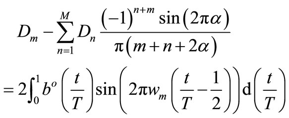 (18)
(18)
Then we use relation 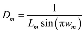 as to calculate Lm of compensator branches.
The offset α in (17) must be less then 0.5 as to assure Lp positive.
4. Frequency-Domain Compensator Design
The frequency-domain approach is a well known method (see M. Pasko [4-6]).
The counterpart of (6) in frequency-domain is
 (19)
(19)
where:
 ,
, —frequency response of compensator and receiver susceptances,
 —harmonic number.
For the elementary compensator branch (LC in series) the branch elementary susceptance is
Thus the formula of reactances balance (19) (see Figures 6 and 7) takes form
 (20)
(20)
The Equation (20) is the counterpart of (11) transformed to optimization task (18).
Then in the particular case of the RL in series receiver we get the set of M linear equations for all Lm of compensator branches
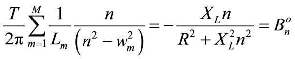 (21)
(21)
where n—harmonic numberm—branch number.
Comparing (18) with (21) we can see that both formulas are the system of linear equations, but in (18) we have
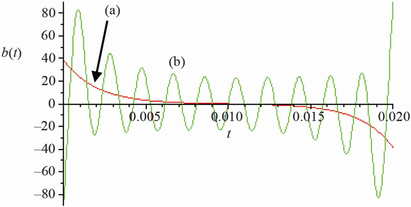
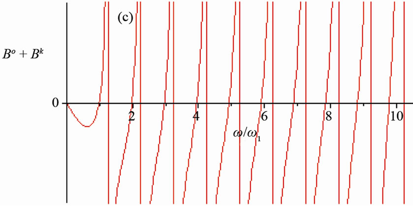
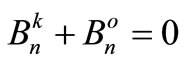
Figure 6. T-periodic time-domain response: (a) Receiver bo(t); (b) Compensator (–bk(t)) and frequency response; (c) Bo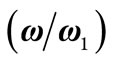 + Bk
+ Bk , for α =
 .
.
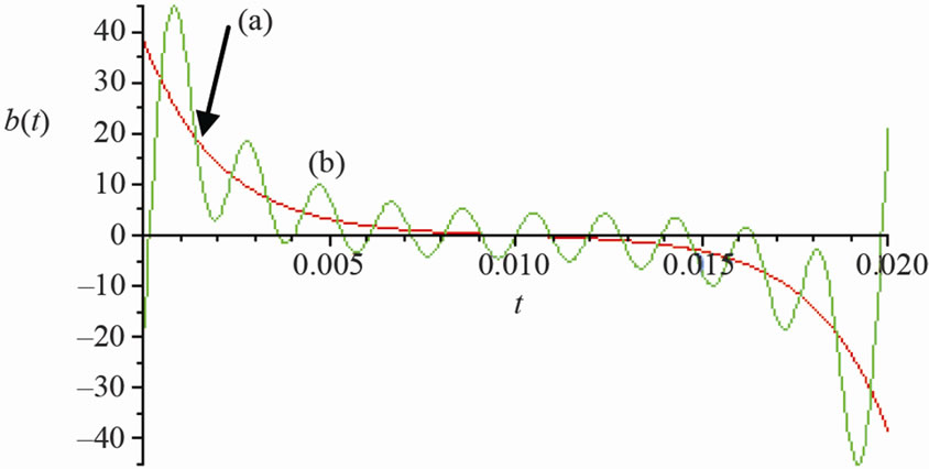
Figure 7. T-periodic time-domain response: (a) Receiver bo(t); (b) Compensator (–bk(t)) and frequency response; (c) Bo + Bk
+ Bk , for α =
 .
.
the impulse response instead of the frequency response of the receiver.
5. Calculation Example
Let consider the RL load in series for which: P = 500 [W], T = 0.02 [s], ω1 = 314 [rad/s], AL = T/τ = 10, Lo = 25.7 [mH] and M = 10, τ—time-constant of the load.
Effective compensation is up to 5-th harmonic (see Figures 6 and 7).
The integral in the right side of (18) was calculated numerically using 21 samples and time samples was shifted by T/21/2 due to singularity problem.
6. Conclusion
The frequency response method used until now to synthesis LC compensators and considered the only one [1], has its counterpart in time-domain. In both approaches the LC parameters can be found with simple optimization techniques for linear system. The only difference is that in (18) we can use directly the impulse response of the load (differentiated step response) instead of harmonic analysis. Moreover it is the first time in literature that the time-domain reactive compensator design is presented.
REFERENCES
- L. S. Czarnecki, “Discussion on ‘a Uniform Concept of Reactive Power of Nonsinusoidal Currents in a TimeDomain’,” Electrical Review, Vol. 85 No. 6, 2009, CDROM.
- M. Siwczyński and M. Jaraczewski, “The L1-Impulse Method as an Alternative to the Fourier Series in the Power Theory of Continues Time Systems,” Bulletin of the Polish Academy of Science, Technical Sciences, Vol. 57, No 1, 2009, pp. 79-86.
- M. Siwczyński, “Decompositions: Active Current, Scattered Current, Reactive Current in Time-Domain—Single-Phase Circuits,” Electrical Review, Vol. 6, 2010, pp. 11-17.
- M. Pasko, “Choice of the Two-Terminal Components, Compensating Reactive Current Component of the Linear Load Fed with Distorted Voltage,” Seminarium z Podstaw Elektrotechniki i Teorii Obwodow, Gliwice-Wisła, 20-23 May 1992, CD-ROM.
- M. Pasko, “Improvement of the Working Conditions of the Real Distorted Voltage Sources Using Two-Terminal LC components,” Scientific Notebook of the Silesium University of Technology Electrotechniques, Vol. 117, 1991, pp. 45-62.
- M. Pasko and J. Walczak, “Optimization of the Power Quality Coefficients of the Electrical Circuits with Nonsinusoidal Periodic Signals,” Wydawnictwo Politechniki Śląskiej, Gliwice, 1996.