Journal of Modern Physics
Vol.4 No.11A(2013), Article ID:39714,8 pages DOI:10.4236/jmp.2013.411A001
Weak Values Influenced by Environment
Graduate School of Humanities and Sciences, Ochanomizu University, Bunkyo-ku, Japan
Email: ban.masashi@ocha.ac.jp
Copyright © 2013 Masashi Ban. This is an open access article distributed under the Creative Commons Attribution License, which permits unrestricted use, distribution, and reproduction in any medium, provided the original work is properly cited.
Received August 24, 2013; revised September 25, 2013; accepted October 24, 2013
Keywords: Weak Value; Quantum Measurement; Decoherence
ABSTRACT
A weak value of an observable is studied for a quantum system which is placed under the influence of an environment, where a quantum system irreversibly evolves from a pre-selected state to a post-selected state. A general expression for a weak value influenced by an environment is provided. For a Markovian environment, the weak value is calculated in terms of the predictive and retrodictive density matrices, or by means of the quantum regression theorem. For a nonMarkovian environment, a weak value is examined by making use of exactly solvable models. It is found that although the anomalous property is significantly suppressed by a Markovian environment, it can survive a non-Markovian environment.
1. Introduction
One of the most characteristic features of quantum mechanics lies in a measurement process which provides some information about an observable of a quantum system to be measured [1]. When an appropriately prepared measuring device is strongly coupled to a system, we can obtain one of eigenvalues, say a, of a measured observable  from the value exhibited by a pointer observable of the measuring device. The result
  is obtained with probability
 , where
  is an initial state of the measured system and
  is the corresponding eigenstate of
 . When we perform measurement on an ensemble of identically prepared systemswe derive the average value
  of the observable from the measurement outcomes. It is obvious that the average value lies inside the spectral range of the observable
 . Hence what we can obtain by quantum measurement is the eigenvalue and average value of the observable. However this is not only the story. In a usual measurement process, the measured system is not referred after the interaction with the measuring device, though it is prepared in an initial state before the interaction. Only the pre-selection of the system is performed. In 1988, Aharonov, Albert and Vaidman [2] have found that if an interaction between a system and a measuring device is sufficiently weak and the measured system is post-selected in a state
  after the interaction with the measuring device, the weak value
  of an observable
  can be obtained from the measurement outcomes. It is surprising that the weak value may take a complex value or a value outside the range of the eigenvalues of an observable. After the discovery of the weak value of an observable, many works have been performed for understanding and generalizing weak values [3-14], and furthermore the weak value has been observed experimentally [15,16].
In the most of the previous works on weak values, dynamics or time evolution of a system to be measured has been neglected. Only the interaction Hamiltonian between a system and a measuring device has been taken into account. However, since a measured system in a real world is unavoidably influenced by an environment, we have to consider the effect of the environment on the weak value as well as intrinsic dynamics of the system. Hence it is interesting to investigate the decoherence of weak values during the irreversible time evolution of a system from pre-selected state to a post-selected state. The irreversible time evolution of a system caused by an interaction with an environment is usually studied by means of the quantum master equation [17,18]. However, the post-selection of the system that is essential for weak values makes it very difficult to investigate the irreversible time evolution by the usual method when an environment is non-Markovian. Therefore, in this paper, we will consider the effect of the irreversible time evolution of the system on the weak value of an observable. In Section 2, we provides a general expression of a weak value during the irreversible time evolution of a quantum system between preand post-selection. We will find that the weak value can be calculated by the quantum master equation or by the quantum regression theorem [18] when the environment is Markovian. To investigate the weak value in the case of a non-Markovian environment, we consider the stochastic dephasing in Section 3 and the single excitation multi-mode Jayes-Cummings model in Section 4, where we can obtain the exact expressions of the weak values in both cases. We provide a brief summary in Section 5.
2. Dynamics of Weak Values Influenced by Environment
We suppose that a quantum system to be measured is placed under the influence of an environment and is initially prepared or pre-selected in a quantum state  at time
 . When there is no initial correlation between them, the equality
  holds, where
  is an equilibrium state of the environment. To measure a system observable
 , we prepare a measuring device in an appropriate quantum state
 . The interaction Hamiltonian between the system and the measuring device is assumed to be
  , where
  stands for the measurement time and
  is a momentum operator of the measuring device, which is canonically conjugate to a position operator (a pointer observable)
 . The system and environment evolve until the measurement is performed at time
  while the measurement device remains unchanged. We denote as
  the unitary operator which describes such time evolution. Then the quantum state of the total system just before the measurement is given by the density operator
 and it becomes
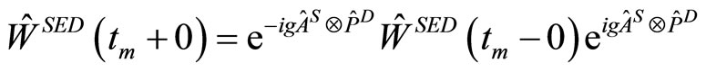 just after the interaction with the measuring device. After the interaction, the system and environment further evolves until the post-selection is performed on the system at time
 . Hence we obtain the quantum state just before the post-selection,
 (1.1)
(1.1)
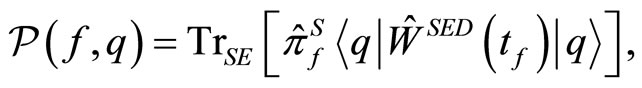
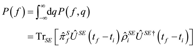
The post-selection performed on the system is, in general, described by means of probability operatorvalued measure which is denoted as . We obtain the joint probability that the post-selection is succeeded and the measuring device exhibits the value q of the pointer observable
 ,
,
 (1.2)
(1.2)
where  is the eigenstate of the pointer observable such that
  and
and  stands for the trace operator over the Hilbert spaces of the system and the environment. Using the Bayes theorem [19], the conditional probability that the measurement outcome is
  if the post-selection is succeeded becomes
 (1.3)
(1.3)
with
 (1.4)
(1.4)
When the post-selection is succeeded, the average value  of the pointer observable is given by
 (1.5)
(1.5)
which will yield the weak value of the observable  under the influence of the environment.
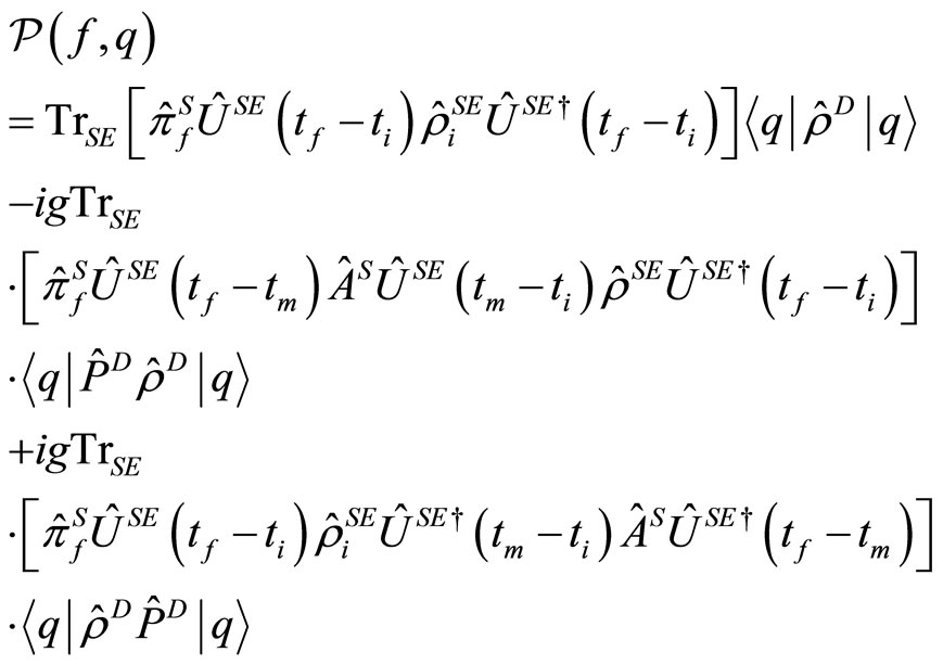
In the weak measurement, the strength of the interaction between the system and the measuring device is sufficiently small and only the terms up to the first order with respect to the coupling constant  is taken into account. Then we obtain from Equation (1.1)
 (1.6)
(1.6)
which yields the joint probability of  and
and  from Equation (1.3),
 (1.7)
(1.7)
When we assume that the probability current density of the measurement device vanishes, the equality holds [6]. Then we obtain after some calculation,
 (1.8)
(1.8)
where  is the weak value of the observable
  influenced by the environment,
 (1.9)
(1.9)
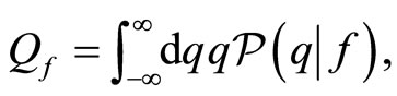
The probability that the post-selection is succeeded is given by
 (1.10)
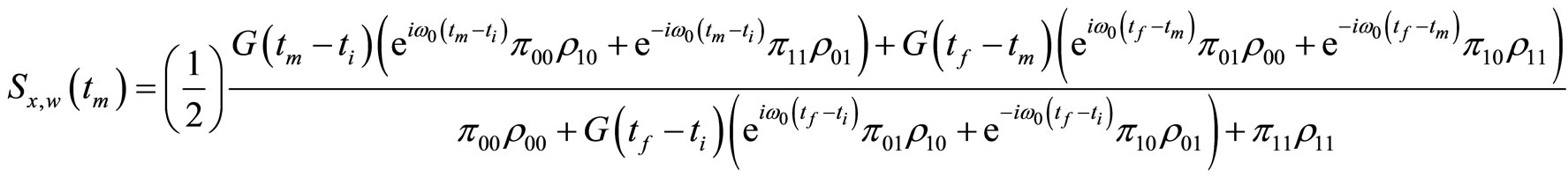
This is independent of the measuring device, which is characteristic of the weak measurement. Thus we obtain the probability of the measurement outcome ,
,
 (1.11)
which yields  with
with 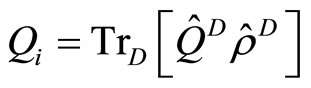 .
.
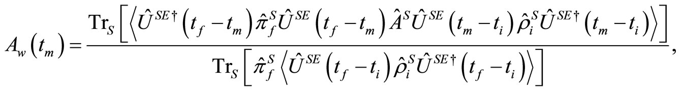
We consider the property of the weak value  given by Equation (1.9). Since the operator
  which represents the post-selection of the system is independent of the environment, the weak value
  becomes
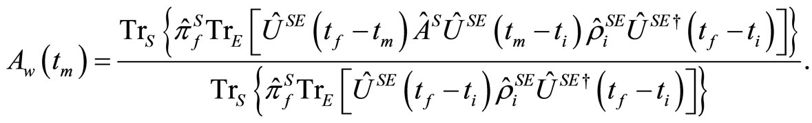 (1.12)
It is obvious that the denominator is the average of the operator  by the reduced density operator
  of the system,
 (1.13)
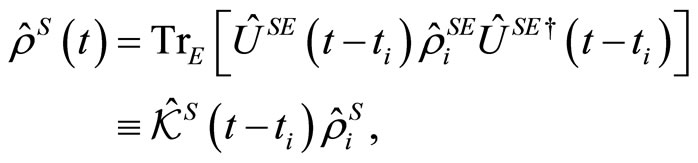
where 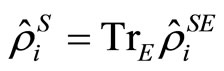 and
and  represents the quantum channel for the system [19]. The reduced density operator
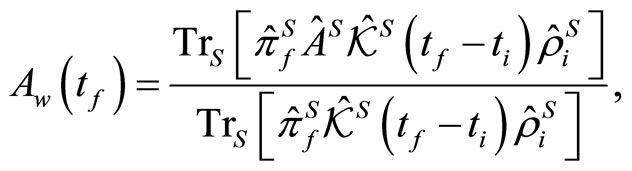
  can be derived by means of the quantum master equation method [17,18]. When the weak measurement is performed just after the pre-selection or just before the post-selection, the weak value is simplified as
 (1.14)
 (1.15)
Thus when  or
or , we can calculate the weak value by means of the quantum channel
  and otherwise calculating the weak value becomes much more difficult.
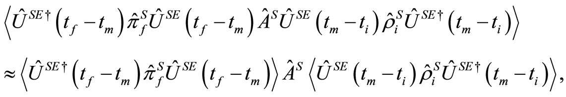
We assume that the environment is Markovian and the influence of the system on the environment is negligible. In this case, the reduced time evolution of the system has the semi-group property [18,20] and we can approximate as [21]
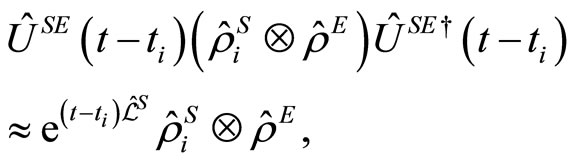 (1.16)
where  represents the equilibrium state of the environment and
  is time evolution generator of the system, which is derived by solving the quantum master equation in a Lindblad form [18,20]. Then we find the weak value from Equation (1.12),
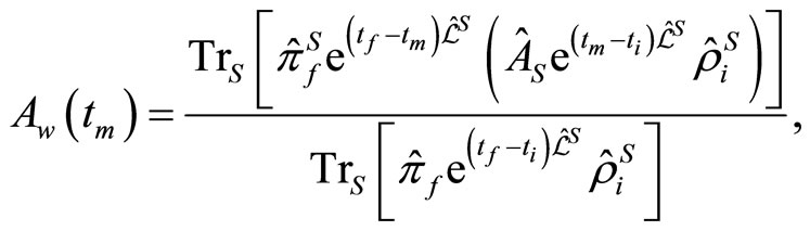 (1.17)
which is equivalent to that obtained by the quantum trajectory method [5]. Using the conjugate of the time evolution generator  defined by
 for any system operators
  and
and , we can express the weak value as
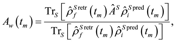 (1.18)
where  and
and  are the predictive and retrodictive density matrices of the system [21],
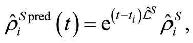 (1.19)
 (1.20)
which are derived by solving the predictive and retrodictive quantum master equations. On the other hand, since we have
 (1.21)
we obtain the weak value,
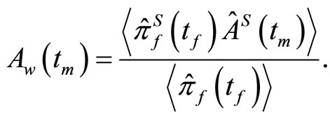 (1.22)
Then if the environment is Markovian, using the quantum regression theorem [18], we can calculate the weak value. Hence we can investigate the weak value influenced by the Markovian environment by Equations (1.17), (1.18) and (1.22). For the non-Markovian environment, however, these results cannot be used and the calculation becomes much more difficult.
3. Weak Values in Stochastic Dephasing
In this section, using an exactly solvable model, we investigate the weak value of an observable influenced by a non-Markovian environment. For this purpose, we use the Kubo-Anderson model [22,23], where the quantum system to be measured is a two-level system or a qubit and the environment causes the stochastic dephasing of the system [24]. The time evolution of the system is governed by a stochastic Hamiltonian,
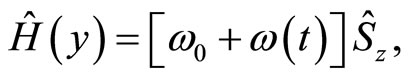 (1.23)
where  is the z-component of a spin-1/2 and
  is a classical stochastic variable with zero mean. The unitary operator that describes the time evolution is given by
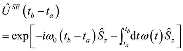 (1.24)
In this case, since the trace operation over the environmental Hilbert space in Equation (1.12) is replaced with the stochastic average, we obtain the weak value of a system observable ,
,
 (1.25)
where  stands for the stochastic average and
  is the initial state of the qubit. Here we note that the approximation given by Equation (1.16) is equivalent to
 (1.26)
which is valid only in the narrowing limit of the dephasing. To calculate the weak value given by Equation (1.25), we expand the initial state , the observable
  and the measurement operator
  as
as  ,
,  and
and , where
  is an eigenstate of
  such that
  and
and . Then after some calculation, we obtain from Equation (1.25),
 (1.27)
with
 (1.28)
and
 (1.29)
where  is the characteristic function of the stochastic variable
 ,
,
 (1.30)
We can see that the approximation given by Equation (1.26) is valid if and only if the equality
 holds or equivalently the characteristic function is given by
 which is derived in the narrowing limit of the dephasing [17]. Assuming that the stochastic dephasing is characterized by the stationary GaussMarkov process, we obtain the characteristic function [17,24],
 (1.31)
while we obtain for the stationary two-state Markov jump process (or equivalently the random telegraph noise) [24,25],
 (1.32)
with . In these equation,
  represents the strength of the dephasing and
  is an inverse of the correlation time of the stochastic variable
 . Note that the Markovian stochastic process does not imply that the dephasing process of the system is Markovian.
Let us now consider the case that the system observable is the  -component
  of the spin. Then the weak value
  given by Equation (1.27) becomes
 (1.33)
In particular, when the system pre-selected in  at the time
  is post-selected in a state
 , the weak value is simplified as
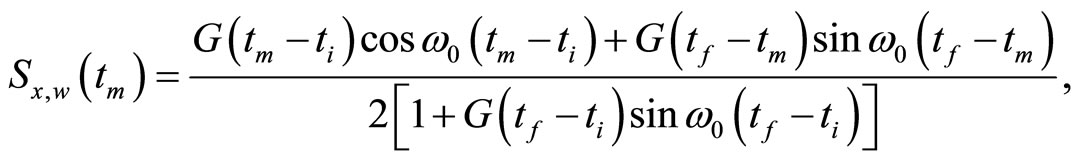 (1.34)
which is plotted as function of time in Figure 1.
It is found from the figure that the weak value lies in the spectral range of the spin-1/2 operator, , in the narrowing limit or equivalently the Markovian limit. This means that the Markovian environment significantly suppresses the anomalous property of the weak value.
4. Weak Value in Bosonic Environment
We consider the weak value influenced by a quantum mechanical environment. Here we suppose that a qubit interacts with an environment consisting of harmonic oscillators [18]. The Hamiltonian of the qubit and environment is given by
 (1.35)
where  and
and  are bosonic annihilation and creation operators of the kth oscillator of the environment. It is assumed that the environment is initially in the vacuum state
  with
with  and it has the Lorentzian spectral density,
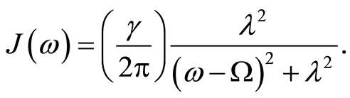 (1.36)
If the inequality 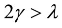 is fulfilled, the environment is non-Markovian and otherwise it is Markovian [18]. We can obtain an exact time evolution of the qubit and the environment. Indeed, when we set the initial state
 with
with , we find the state
  at time
  [18,26],
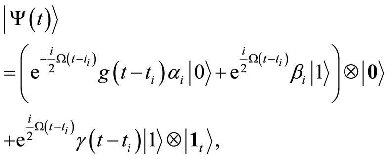 (1.37)
where 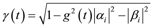 and the time-de-


Figure 1. The weak value of  in the stochastic dephasing which is characterized by (a) the stationary Gauss-Markov process and (b) the stationary two-state-jump Markov process, where the weak measurement is performed at the middle between the pre-selection at
  and the post-selection at
 , that is,
 . We set
  and scale time by the phase relaxation time
  in the narrowing limit, where
  for the Gauss-Markov process and
  for the two-state-jump Markov process. In (a), the solid line (black) stands for
 , the long dashed line (blue) for
 , the short dashed line (brown) for
  and the dotted line (red) for
 . In (b), the solid line (black) stands for
 , the long dashed line (blue) for
 , the short dashed line (brown) for
  and the dotted line (red) for
 . Furthermore we set
  in the figure.
pendent parameter  is given by
 (1.38)
with . In Equation (1.37), we set
 , where the coefficient
  is given by
 (1.39)
Then the exact time evolution of the qubit and the environment is provided by Equations (1.37)-(1.39).
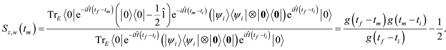
To find how the weak value is influenced by the bosonic environment, we suppose that the observable is the z-component of the spin-1/2 operator and the qubit is post-selected in the excited state  at time
 . Then if
 , we can derive the weak value from Equations (1.12) and (1.37), please see Equation (1.40) below.
It is interesting to note that the weak value does not depend on  and
and . In other words, the weak value is independent of the pre-selection of the system. If the bosonic environment is Markovian
 , we see that
  since the equality
 is satisfied. If the equality
  holds, we obtain
 (1.41)
which yields the inequality . In this case, the weak value is always greater than the maximum eigenvalue of the spin-1/2 operator
 . Furthermore, if the inequality
  is fulfilled, the weak value
  can take values inside and outside the spectral range of the spin-1/2 operator since
  becomes an oscillatory function,
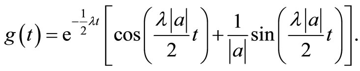 (1.42)
 (1.40)
When  is sufficiently small, the weak value becomes large, though the success probability of the post selection is very small. The time dependence of the weak value is plotted in Figure 2.
5. Summary
In this paper, we have considered the weak value of an
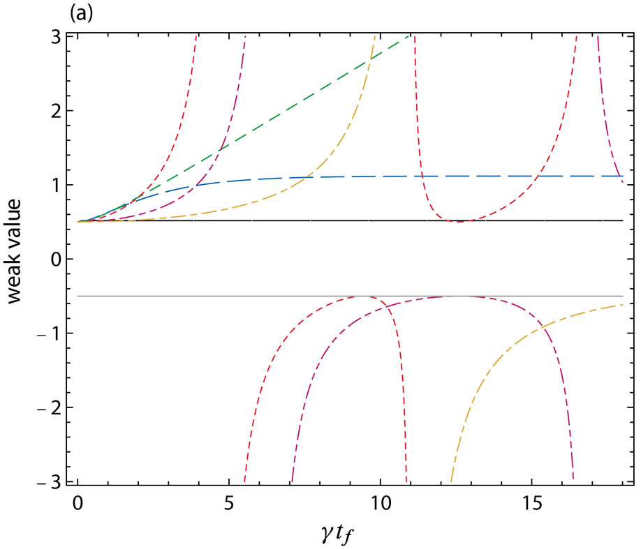
Figure 2. The weak value of  influenced by the bosonic environment, where (a) shows the dependence on the post-selection time in the case of
  and
and , and (b) is the dependence on the measurement time when
  and
and . In both figures, the solid line (black) stands for
 , the long dashed line (blue) for
 , the short dashed line (green) for
 , the dotted line (red) for
  the double dot-dashed line (purple) for
  and the dot-dashed line (brown) for
 . The horizontal gray line in (a) represents
  for reference.
observable of a system interacting with an environment and we have provided the general expression of the weak value influenced by an environment. Since the post-selection of the system is performed, it is, in general, very difficult to calculate the weak value. When the environment is Markovian, we can obtain the weak value in terms of the predictive and retrodictive density matrices of the system, which are derived by solving the quantum master equations, or by means of the quantum regression theorem. On the other hand, for the non-Markovian environment, we don’t know the systematic method for calculating weak values. Hence to investigate the weak value in the case of the non-Markovian environment, we have applied the two exactly solvable models. One is the stochastic dephasing model and the other is the single excitation multi-mode Jayes-Cummings model. We have found that the Markovian environment significantly suppresses the anomalous behavior of the weak value in comparison with the non-Markovian environment. Since we have used the specific models, we have to consider more general cases. For this purpose, however, it is necessary to develop a method for calculating weak values under the influence of the environment.
6. Acknowledgements
The author would greatly appreciate Prof. F. Shibata and Prof. S. Kitajima for their stimulating discussions.
REFERENCES
- J. Von Neumann, “Mathematical Foundations of Quantum Mechanics,” Princeton University Press, New Jersey, 1955.
- Y. Aharonov, D. Z. Albert and L. Vaidman, Physical Review Letters, Vol. 60, 1988, pp. 1351-1354. http://dx.doi.org/10.1103/PhysRevLett.60.1351
- I. M. Duck, Physical Review D, Vol. 40, 1989, pp. 2112- 2117. http://dx.doi.org/10.1103/PhysRevD.40.2112
- Y. Aharonov and L. Vaidman, Physical Review A, Vol. 41, 1990, pp. 11-20. http://dx.doi.org/10.1103/PhysRevA.41.11
- H. M. Wiseman, Physical Review A, Vol. 65, 2002, Article ID: 032111.
- L. M. Johansen, Physical Review Letters, Vol. 93, 2004, Article ID: 120402. http://dx.doi.org/10.1103/PhysRevLett.93.120402
- L. M. Johansen and A. Luis, Physical Review A, Vol. 70, 2004, Article ID: 052115. http://dx.doi.org/10.1103/PhysRevA.70.052115
- L. M. Johansen, Physical Letters A, Vol. 322, 2004, pp. 298-300. http://dx.doi.org/10.1016/j.physleta.2004.01.041
- R. Jozsa, Physical Review A, Vol. 76, 2007, Article ID: 044103. http://dx.doi.org/10.1103/PhysRevA.76.044103
- A. C. Lobo, Physical Review A, Vol. 80, 2009, Article ID: 012112. http://dx.doi.org/10.1103/PhysRevA.80.012112
- T. Geszti, Physical Review A, Vol. 81, 2010, Article ID: 044102. http://dx.doi.org/10.1103/PhysRevA.81.044102
- X. Zhu, Y. Zhang, S. Pang, C. Qiao, Q. Liu and S. Wu, Physical Review A, Vol. 84, 2011, Article ID: 052111.
- S. Wu and Y. Li, Physical Review A, Vol. 83, 2011, Article ID: 052106.
- A. G. Kofman, S. Ashhab and F. Nori, Physics Report, Vol. 520, 2012, pp. 43-133. http://dx.doi.org/10.1016/j.physrep.2012.07.001
- P. B. Dixon, D. J. Starling, A. N. Jordan and J. C. Howell, Physical Review Letters, Vol. 102, 2009, Article ID: 173601. http://dx.doi.org/10.1103/PhysRevLett.102.173601
- D. J. Starling, P. B. Dixon, A. N. Jordan and J. C. Howell, Physical Review A, Vol. 82, 2010, Article ID: 063822.
- R. Kubo, M. Toda and N. Hashitsume, “Statistical Physics II,” Springer, Berlin, 1985. http://dx.doi.org/10.1007/978-3-642-96701-6
- H. Breuer and F. Petruccione, “The Theory of Open Quantum System,” Oxford University Press, Oxford, 2006.
- M. A. Nielsen and I. L. Chuang, “Quantum Computation and Quantum Information,” Cambridge University Press, Cambridge, 2000.
- R. Alicki and K. Lendi, “Quantum Dynamical Semigroups and Applications,” Springer, Berlin, 2007.
- S. M. Barnett, D. T. Pegg, J. Jeffers and O. Jedrkiewicz, Physical Review Letters, Vol. 86, 2001, pp. 2455-2458. http://dx.doi.org/10.1103/PhysRevLett.86.2455
- P. W. Anderson, Journal of the Physical Society of Japan, Vol. 9, 1954, pp. 316-339. http://dx.doi.org/10.1143/JPSJ.9.316
- R. Anderson, Journal of the Physical Society of Japan, Vol. 9, 1954, pp. 935-944. http://dx.doi.org/10.1143/JPSJ.9.316
- M. Ban, S. Kitajima and F. Shibata, Physics Letters A, Vol. 349, 2006, pp. 415-421. http://dx.doi.org/10.1016/j.physleta.2005.09.062
- N. G. van Kampen, “Stochastic Processes in Physics and Chemistry,” Elsevier, Amsterdam, 1981.
- M. Ban, S. Kitajima and F. Shibata, Physics Letters A, Vol. 375, 2011, pp. 2283-2290. http://dx.doi.org/10.1016/j.physleta.2011.04.049