ABSTRACT

Conventional interpretation of the Einstein Equation has inconsistencies and contradictions, such as gravitational fields without energy, objects crossing event-horizons, objects exceeding the speed of light, and inconsistency in scaling the speed of light and its factors. An isotropic metric resolves such problems by attributing energy to the gravitational field, in the Einstein Equation. This paper discusses symmetries of an isotropic metric, including scaling of physical quantities, the Lorentz transformation, covariant derivatives, and stress-energy tensors, and transitivity of this scaling between inertial reference frames. Force, charge, Planck’s constant, and the fine structure constant remain invariant under isotropic gravitational scaling. Gravitational scattering, orbital period, and precession distinguish between isotropic and Schwarzschild metrics. An isotropic metric accommodates quantum mechanics and improves models of black-holes.

1. Introduction

The present interpretation of the Einstein Equation in general relativity has troubling inconsistencies and contradictions, such as violation of semiclassical locality, quantum unitarity, time reversibility, and energy conservation [1]. For example, when an object crosses a Swarzschild black-hole’s event-horizon, it attains the speed of light, giving the object unbounded energy for nearby observers. Apparently, conservation of energy must be grossly violated, at least for local observers near the event-horizon. Since the Einstein Equation explicitly conserves energy, then the Einstein Equation must not work for local observers. Conventionally, one assumes that the Einstein Equation works only for distant observers, but by their location within the massive cosmos, all physical observers are local observers. So, the present interpretation of the Einstein Equation does not work for any physical observer. Moreover, a rotating black-hole can have a naked singularity, resulting in contradictions of time-travel [2]. Since the conventional model of a black-hole predicts objects to enter a region where the model no longer makes sense, then something must be lacking from the model.

Since the Einstein Equation is designed to conserve energy, the failure to conserve energy must involve application of the equation, such as the failure to account for the energy density of the gravitational field. When one assembles electric charges on a sphere, one applies a force through a distance on the charges, and thus puts energy into the electric field. For gravity, ordinary mass plays the role of charge. When one assembles a sphere of mass, energy is released. So, a gravitational field should have negative energy density. The Einstein Equation equates, which is a contraction of the curvature tensor for space-time, to, which is the local energy and momentum density. The fact that the conventional Schwarzschild metric for a black-hole is derived by solving the differential equations for for all regions around the singularity, implies that the gravitational fields have no energy nor momentum.

The resulting Schwarzschild metric for a black-hole is anisotropic: While objects in the gravitational well look shorter in a radial direction, their azimuthal dimensions remain unaffected, as viewed by a remote observer. Then, the speed of light is also anisotropic, and one cannot consistently scale mass and energy, and complications arise in reconciling gravity with quantum mechanics. These contradictions and inconsistencies should inspire us to consider a different metric.

2. Isotropic Metric

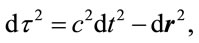
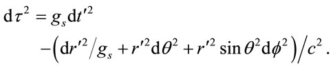
An isotropic metric with the scaling for time reciprocal that for space, yields a distance differential, in terms of a distant observer’s coordinates:

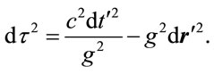(1.1)

The speed of light as seen from a distance, , in terms of that locally, , is 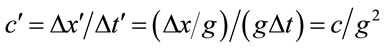, which means that since, light in a gravitational well moves more slowly. As a result, a gravitational field deflects light. Therefore, this metric is not “conformally flat”. Because the metric is isotropic, objects no longer cross eventhorizons. For example, one can see that in the orbit Equation (1.44) below, for a spherically symmetric potential, is bounded.

In matrix form for spherical coordinates, this isotropic metric is

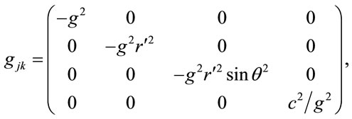(1.2)

so that the length differential

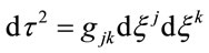(1.3)

is that in Equation (1.1). The term of the Einstein Tensor equals the total energy density. For an isotropic metric, it has two terms, one that has the form of a charge density, and the other that has the form of an energy density of a field [3]:

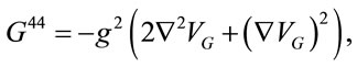(1.4)

where 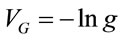is the gravitational potential in terms of scale factor. One should ascribe the energy density of ordinary matter to the first term of the Einstein Tensor, and the energy density of the gravitational field to the second term. In the course of deriving this form, one finds that the metric scales momentum-energy like it scales space-time. Mass differential

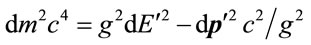(1.5)

corresponds to distance differential in Equation (1.1) above.

Explicit inclusion of factors of c helps to verify scaling factors of g in these equations. Unlike the isotropic metric in Equation (1.1), isotropic metrics rejected in the past were conformally flat. They also did not include the corresponding relation (1.5) for momentum and energy, nor the energy of gravitational fields in the Einstein Tensor (1.4). While the same isotropic metric by Yilmaz [4] has an implicit globally preferred reference frame due to flawed assumptions ancillary to the form of the metric, the gravitational fields for the metric here have rest frames that vary from point to point, as shown in Equation (1.21) below. Such rest frames are consistent with frame-dragging. The “Parameterized Post-Newtonian” (PPN) parameters for equation (0.1) as defined on pp. 1084-1085 of Gravitation [5] are:., , , , , , , , , , ,. The nonzero value for is consistent with the existence of rest frames, although there is no globally preferred frame.

For a point source without rotation, metric scaling [3]

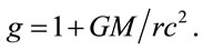(1.6)

Since this scaling appears in the metric as 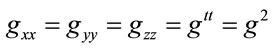, it is the same as Schwarzschild metric 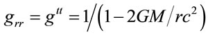to first order in the gravitational constant, but differs greatly in the strong field limit. For example, the event-horizon is at for an isotropic metric. So, one must look at strong gravitational fields to distinguish between them.

3. Scaling of Physical Quantities

It would help to consider scaling of physical quantities, to avoid blunders in gravitational scaling, and to identify those quantities that are invariant. Suppose a local observer in a gravitational field measures the distance between events, and a remote observer external to the gravitational field measures the distance between the same two events. In local coordinates,

(1.7)

while in remote coordinates,

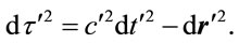(1.8)

In terms of remote coordinates, and . These substitutions into Equation (1.7) give the distance differential (1.1) from which one may infer the metric tensor, and calculate the affine connection and Einstein Tensor. Substitution into Equation (1.1) yields, which shows that scaling is transitive for successive reference frames:

(1.9)

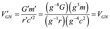
Scale factor grows to values greater than one, toward an attractive gravitational potential. So, shows that, as seen by a remote observer, an object in a gravitational well is shorter. For time,; energy,; momentum,; energy density; and mass,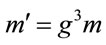. Force and angular momentum are invariant. So, all observers agree on the value of.

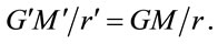
The gravitational constant scales as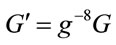. To change the scaling of a physical quantity, one can multiply by powers of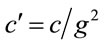. For example, the dimensionless quantity in,

(1.10)

is invariant under scaling. By redistributing powers of, is invariant under scaling, and scales like energy.

To preserve the symmetry of the Helmholtz-Maxwell Equations, the electric permittivity and magnetic permeability scale the same way. Then

(1.11)

shows and. Energy density of an electromagnetic field,

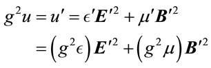(1.12)

shows that and. Also, shows that electric charge, and fine structure constant 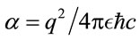are invariant.

4. Scaling in a Lorentz Transformation

Although the metric is Lorentz invariant in the local reference frame, where scaling, it is not Lorentz invariant for all observers. With proper choice of coordinates, a Lorentz transformation of a vector is

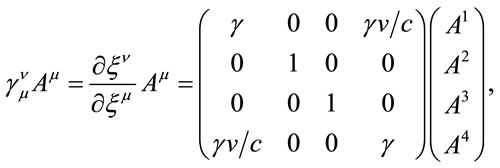(1.13)

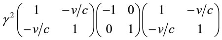
where the Lorentz scaling is

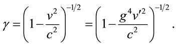(1.14)

To simplify display in the rest of this section, dimensions not affected by a Lorentz transformation will not be displayed. Then a Lorentz transformation and its inverse are

(1.15)

(1.16)

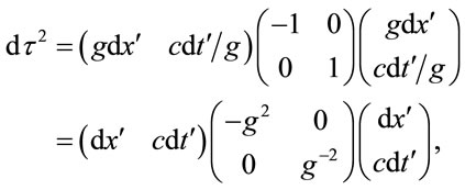
While the metric is not Lorentz invariant for all observers, the length differential is, when written in the form

                                        (1.17)

Insertion of the Lorentz transformation and its inverse shows the Lorentz invariance of the length differential,

                                      (1.18)

where, , , and are all the same Lorentz transformation. Then the Lorentz transformed metric

(1.19)

is Lorentz invariant. But, in remote coordinates, Equation (1.17) becomes,

(1.20)

where in the last step, the scaling transfers from the coordinates to the metric tensor. Insertion of a Lorentz transformation and its inverse, in remote coordinates, shows that the Lorentz transformed metric is

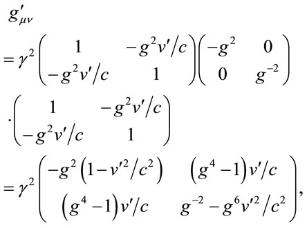(1.21)

yielding a length differential in expected form in remote coordinates,

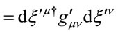
                                        (1.22)

Under a Lorentz transformation, the metric loses its isotropy, and acquires off-diagonal terms. Diagonalization generates the Lorentz transformation back to the local rest frame of the gravitational field, where the metric scaling factor appears like an eigenvalue.

5. Scaling in Stress Tensors

Covariant differentiation of vector,

(1.23)

takes into account both the change in, in, and an additional apparent transformation of in the curved space, in, where the Christoffel symbol for the affine connection is

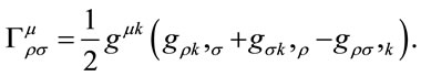(1.24)

For example, the covariant derivative in the y-direction of a vector along the -direction is is

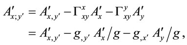(1.25)

If one divides through by,

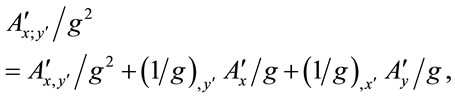(1.26)

then the equation takes a form where the terms are scaled to the local observer’s coordinates, plus a rotation:

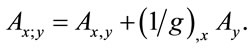(1.27)

So, covariant differentiation implicitly accounts for scaling.

Since, in the Dirac Equation, the electromagnetic vector potential couples to fermion momentum and energy, as in, and since charge is unaffected by scaling, then each component of the vector potential should scale like the operator to which it couples. For example, scales like momentum. The electromagnetic field tensor in covariant form

(1.28)

contravariant form,

(1.29)

and mixed form

(1.30)

all appear in the electromagnetic stress tensor

(1.31)

If a gravitational field is present, then one should use covariant differentiation, to account for curved space. As shown above, covariant differentiation also accounts for scaling.

(1.32)

To preserve the symmetry of Equation (1.28), which suppresses factors of, and to keep scaling consistent for the two terms of, one can require to couple to, instead of the energy operator alone, so that all components of the vector potential scale like momentum. In the same way, any other derivative with respect to time should be divided by a factor of, to scale it like derivatives with respect to space. Then, and for all diagonal components of the metric. Since, scales like momentum, then and. Likewise, since , then, and. One should expect to scale like an energy density. The scaling for the forms of suggest that scales as. The implicit factors, which are the permitivity and permeability, scale as, as shown above in Equation (1.11). Therefore, to get the expected scaling for, one should also divide by a factor of.

6. Orbit Equation for an Isotropic Metric

Recently, long-lived stars have been found orbiting the black-hole in the center of the Milky Way galaxy, in unexpectedly small orbits [6,7]. Measurement of the precession of orbits might make it possible to distinguish between a Schwarzschild metric and an isotropic metric, especially if one can observe an orbit smaller than the Schwarzschild radius. Furthermore, for an isotropic metric, non-decaying orbits exist at all distances from a black-hole.

As usual, equations of motion are

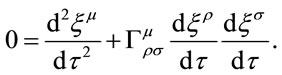(1.33)

For in Equation (1.33),

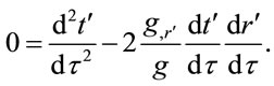(1.34)

Integration yields a constant of motion

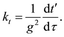(1.35)

This scaling might seem to contradict evident in (1.1), but the scaling in (1.35) describes a curved orbit, while that in (1.1) describes a straight-line distance. From (1.1),

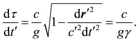(1.36)

Substitution of this into (1.35) shows that along an orbit,

(1.37)

Special and general relativistic effects have the same magnitude. The orbiter’s energy and the remote observer’s metric determine constant of motion.

Application of Equation (1.33) to, the polar angle, yields

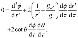(1.38)

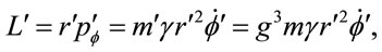
With choice of coordinates such that, this equation integrates to a constant of motion that is the angular momentum,

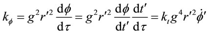(1.39)

Again, scaling for this constant is reconciled to invariant angular momentum,

(1.40)

by substitution. While all observers agree on the angular momentum of a particle, the contribution of the particle to the total angular momentum varies over its orbit, since its rest mass does not change while it traverses different values of the metric.

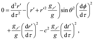
For in Equation (1.33),

(1.41)

which reduces to

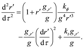(1.42)

Integration of this equation gives

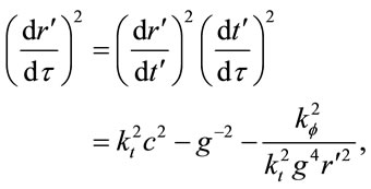(1.43)

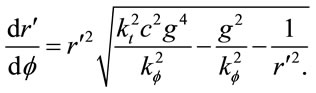
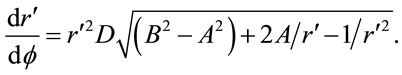
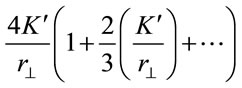
where

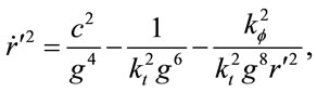(1.44)

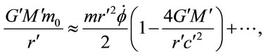
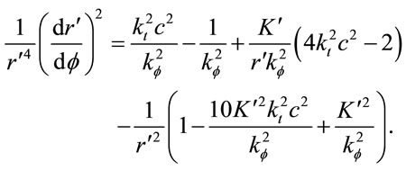
which is an expansion of Equation (1.37),. At sufficiently small, the negative terms of Equation (1.44) make. Unlike the Schwarzschild metric, stable orbits exist at all radii for an isotropic metric. Multiplication of Equation (1.43) by gives an effective potential in the Newtonian approximation.

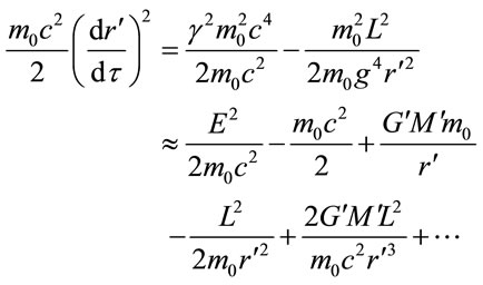(1.45)

to first order in. The last term comes from the harmonic expansion

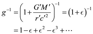(1.46)

Expansion (1.45) first differs from that for a Schwarzschild metric in the factor of two on the last term. So, correction to the orbital period for an isotropic metric is twice that for a Schwarzschild metric. Since, ,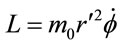

(1.47)

which then yields

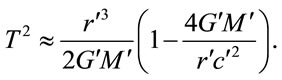(1.48)

The ratio from Equations (1.39) and (1.44) gives the orbit equation

(1.49)

With expansion to of powers of 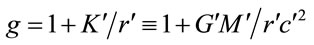, Equation (1.49) becomes

(1.50)

For the Newtonian approximation, 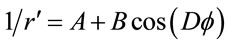, where, , and, are constants to be determined,

(1.51)

Comparison of the above two equations shows that. The precession is 50% larger than that given for a Schwarzschild metric. The comparison would be complicated by rotation of the gravitational field.

For scattering,. For a massless particle at this limit, , because g is one; and , where is the impact parameter and is the initial speed. For a small deflection, in this limit,.

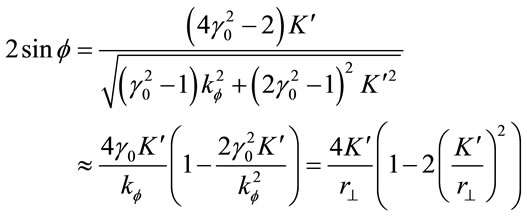(1.52)

for an isotropic metric, versus

(1.53)

for a Schwarzschild metric.

7. Inconsistency for a Schwarzschild Metric

The Schwarzschild metric has inherent inconsistencies, mostly due to neglecting to scale the speed of light. For the Schwarzschild metric,

(1.54)

As already explained, primed quantities are distant measures, while unprimed are local measures. For a point source, the Schwarzschild metric scaling

(1.55)

where is one. The standard interpretation assumes that all observers agree on the metric. Therefore

(1.56)

To relate the gravitational potential energy of a system, as measured locally, to that measured remotely, suppose, as an ansatz, that energy scales as

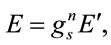(1.57)

where is yet to be determined. Then

(1.58)

With the scaling for for radial motion,

(1.59)

With scaling for for azimuthal motion,

(1.60)

Substitution for into Equation (1.58), from Equation (1.59) yields

(1.61)

Then substitution into Equation (1.56) shows that gravitational potential energy scales as

(1.62)

The scaling of this gravitational energy contradicts that in Equation (1.57). The scaling for in Equation (1.60) has the same problem. Therefore the Schwarzschild metric implies a preferred remote frame of reference in which physics is self-consistent; one cannot use potentials to conserve momentum and energy in any physical reference frame. In contrast, an isotropic metric has selfconsistency across all inertial frames of reference, as shown by Equation (1.9).

8. Conclusion

That an isotropic metric accounts for the energy of a gravitational field, should be sufficient reason to adopt an isotropic metric over a Schwarzschild metric. Further reason is provided by the symmetries of scaling for an isotropic metric, such as that between the length differential and the mass-energy-momentum equation. The invariance under isotropic scaling of force, angular momentum, electric field, electric charge, and fine structure constant provide consistency of general relativity with both quantum mechanics and electromagnetism. Orbits no longer cross event horizons. Inconsistencies in scaling for a Schwarzschild metric make the Schwarzschild metric untenable, necessitating adoption of the isotropic metric.

9. Acknowledgements

The author thanks his parents, his brother David Rudmin, and George Gillies for proofreading and encouragement.

REFERENCES

- S. B. Giddings, Physics Today, Vol. 66, 2013, pp. 30-35. doi:10.1063/PT.3.1946
- D. M. Eardley and L. Smarr, Physical Review D, Vol. 19, 1979, pp. 2239-2259. doi:10.1103/PhysRevD.19.2239
- J. D. Rudmin, Virginia Journal of Science, Vol. 58, 2007, pp. 27-33.
- H. Yilmaz, Physical Review, Vol. 111, 1958, pp. 1417- 1426. doi:10.1103/PhysRev.111.1417
- C. W. Misner, K. S. Thorne and J. A. Wheeler, “Gravitation,” W. H. Freeman and Company, San Francisco, 1973.
- T. Alexander, Physics Reports, Vol. 419, 2005, Article ID: 65142.
- R. Genzel and V. Karas, “The Galactic Center,” Proceedings of the International Astronomical Union Symposium, Prague, 21-25 August 2007, pp. 173-180.