

Applied Mathematics
Vol.06 No.10(2015), Article ID:59455,10 pages
10.4236/am.2015.610148
The Dynamic Properties of a Deterministic SIR Epidemic Model in Discrete-Time
Xiaodan Liao, Hongbo Wang, Xiaohua Huang, Wenbo Zeng, Xiaoliang Zhou*
Department of Mathematics, Lingnan Normal University, Zhanjiang, China
Email: *zxlmath@163.com
Copyright © 2015 by authors and Scientific Research Publishing Inc.
This work is licensed under the Creative Commons Attribution International License (CC BY).
http://creativecommons.org/licenses/by/4.0/



Received 2 May 2015; accepted 5 September 2015; published 8 September 2015
ABSTRACT
In this paper, a class of discrete deterministic SIR epidemic model with vertical and horizontal transmission is studied. Based on the population assumed to be a constant size, we transform the discrete SIR epidemic model into a planar map. Then we find out its equilibrium points and eigenvalues. From discussing the influence of the coefficient parameters effected on the eigenvalues, we give the hyperbolicity of equilibrium points and determine which point is saddle, node or focus as well as their stability. Further, by deriving equations describing flows on the center manifolds, we discuss the transcritical bifurcation at the non-hyperbolic equilibrium point. Finally, we give some numerical simulation examples for illustrating the theoretical analysis and the biological explanation of our theorem.
Keywords:
Epidemic Model, Equilibrium Point, Transcritical Bifurcation, Center Manifold, Hyperbolicity

1. Introduction
Since Kermack and McKendrick [1] proposed the Susceptible-Infective-Recovered model (or SIR for short) in 1927, a lot of glorious studies on the dynamics of the epidemic models have been presented (see [2] -[9] ). The basic and important research subjects for these systems are local and global stability of the disease-free equilibrium and the endemic equilibrium, existence of periodic solutions, persistence and extinction of the disease, etc. According to the dependence on variable (i.e., time), these systems were classified into two types: continuous- time system and discrete-time system.
For the epidemic models, there have been a lot of researches focusing on the case of continuous-time (see [2] -[6] and that cited therein). However, discrete-time models (or called difference equations) are also useful for modeling situations of epidemic. They can not only have the basic features of the corresponding continuous- time models but also provide a substantial reduction of computer time (see [10] ). What is more, a lot of discrete- time models are not trivial analogues of their continuous ones and simple models can even exhibit complex behavior (see [5] [10] ).
In 1989, Hethcote [7] considered a class of continuous epidemic model with vertical and horizontal transmission.
 (1)
(1)
where S represents the proportion of individuals susceptible to the disease, who are born (with b) and die (with d) at the same rate b (b = d), and have mean life expectancy 1/b. The susceptible becomes infectious at a bilinear rate βI, where I is the proportion of infectious individuals and β is the contact rate. The infectious recover (i.e., acquire lifelong immunity) at a rate r, so that 1/r is the mean infectious period. The constant p, q,  ,
,  , and
, and , where p is the proportion of the offspring of infective parents that are susceptible individuals, and q is the proportion of the offspring of infective parents that are infective individuals. Because of biological meanings, a natural constraint is
 . A similarly detailed description of the model and its dynamics may be found in [7] . In recent, Meng and Chen [8] have also studied the epidemic system (1). In their work, the basic reproductive rate determining the stability of disease-free equilibrium point and endemic equilibrium point was found out and the local and global stability of the equilibrium points have been researched by using Lyapunov function and Dulac function.
In this paper, we pay attention to the discrete situation of (1). From discussing the influence of the coefficient parameters effected on the eigenvalues, we give the hyperbolicity of equilibrium points and determine which point is saddle, node or focus as well as their stability. Further, by deriving equations describing flows on the center manifolds, we discuss the transcritical bifurcation at the non-hyperbolic equilibrium point and research how does small perturbation of coefficient parameters affect the number and stability of equilibrium points. Moreover, we give some numerical simulation examples for illustrating the theoretical analysis and explain the biological meaning of our theorem.
2. Discrete SIR Epidemic Model with Vertical and Horizontal Transmission
In this section, we consider the discrete SIR epidemic model with vertical and horizontal transmission:
 (2)
(2)
where ,
,  and
and  represent susceptible, infective and removed (or isolated) subgroups respectively, n represents a fixed time,
 . It is assumed that
 ,
,  ,
,  and
and . In view of assumption that population is a constant size in [3] , i.e.,
 (3)
(3)
system (2) can be changed into
 (4)
(4)
Rewrite (4) as a planar map F:
 (5)
(5)
It is obvious that this map has a disease-free equilibrium point  and an endemic equilibrium point
 , where
 ,
,  and
and .
.
The organization of this paper is as follows. In next section, we identify all cases of non- and hyperbolic equilibria, which is a fundament for all succeeding studies. In Section 4, we discuss the transcritical bifurcation at the disease-free equilibrium of (1), the direction and stability of the transcritical bifurcation is investigated by computing a center manifold. In Section 5, some simulations are made to demonstrate our results and the biologic explanation of the theorem is also given.
3. Hyperbolic and Non-Hyperbolic Cases
In this section, we will discuss the hyperbolic and non-hyperbolic cases in a two parameters space parameter.
Theorem 1. The equilibrium point  is non-hyperbolic if and only if
  lies on the lines:

and

Otherwise, the equilibrium point  is in one of the following types (see Table 1).
Remark 1. By Theorem 3.1 the domain  is divided by line
  and
and  into three districts
 ,
,  and
and  for equilibrium point P (see Figure 1).
Proof. The Jacobian matrix of (5) at  is
is

and its eigenvalues are

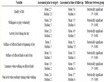
Table 1. Types of hyperbolic equilibrium point .
.

Figure 1. Districts for equilibrium point P.
From the assumption , we see that
 . Then non-hyperbolicity will be happened in the case
 . From
 , we know
  which means
  lies on
 ; Also, From
 , we get that
  and
and  lies on
 . When
  (referred to the case
 ), the eigenvalue
  satisfies
 , then the equilibrium point P is a stable node. When
  (referred to the case
 ), the equilibrium point P is a node since
  and meanwhile when
 , the equilibrium P is a saddle since
 . The proof is complete. □
Theorem 2. There does not exist non-hyperbolic case for equilibrium point . But the hyperbolicity can be divided into the following cases:
(I) When , there exist six types for hyperbolic equilibrium point Q (see Table 2).
Where  and
and  satisfy
 :
:

and :
: , respectively.
(II) When , there exist four types for hyperbolic equilibrium point Q (see Table 3).
Where  satisfies
 :
: .
.
Remark 2. By Theorem 3.2, when , the domain
  is divided by line
 ,
,  and
and  into three districts
 ,
,  ,
,  and
and  for equilibrium point Q (see Figure 2).
When , the domain
  is divided by line
  and
and  into three dis-
tricts ,
,  and
and  for equilibrium point Q (see Figure 3).
Proof. Performing a coordinate shift as follows:

Table 2. Types of hyperbolic equilibrium .
.
Table 3. Types of hyperbolic equilibrium .
.

Figure 2. Districts for equilibrium point Q when b < β.

Figure 3. Districts for equilibrium point Q when b1 < β ≤ b.
and letting  denote the transformed f, we translate equilibrium
  into
into  and discuss equilibrium point
  of the map
 . The matrix of linearization of
  at
at  is
is

where  and
and , and its eigenvalues are
 (6)
(6)
It is known that  is hyperbolic if and only if none of eigenvalues
 ,
,  lies on the unit circle
 . In the following we discuss the eigenvalues in two cases, i.e.,
  and
and .
.
Case (I). When discriminant , then λ1 and λ2 are both real. Because non- hyperbolicity happens if and only if
  or
or  is 1. For whether λ1 = 1 or λ2 = 1, we can get
 . However, for positive equilibrium point Q, we have 0 < a < 1 and 0 < r < 1. Therefore, neither λ1 = 1 nor λ2 = 1 is possible. Next, let’s examine
  and
and . From whether
  or
or , we can get
 . By condition
 ,
,  , we see that
 . This is a contradiction with
 , so
, so  and
and  are impossible.
In the case of ,
,  and
and  are a pair of conjugate complex. Since

 and
and  lie inside of
  and the equilibrium point Q is a stable focus referred to the case
 .
.
If , i.e.,
  , the matrix has a double real eigenvalue
 . From the constraint condition
  of s, it is obvious that
 . Therefore, equilibrium Q is stable node in the cases of
  and
and .
.
If , i.e.
  and
and , the eigenvalues
  and
and  are different real numbers. We first discuss the case that
 , i.e.
 . In this case we have

Since

we have  for
for . On the other hand, there also exists
  for
for . In fact, since

and

we have . Therefore, the equilibrium Q is a stable node as
 .
.
For the case , i.e.,
  , we have

and

Therefore, the equilibrium Q is a stable node as .
.
Finally, we study the case of , i.e.
 . We have

Then, we have  for
for . Moreover, there also has
  for
for . In fact that,

This means that the equilibrium Q is a stable node for .
.
Case (II). When discriminant , then
  and
and  are both real. Because non-hyperbolicity happens if and only if
  or
or  is 1. Similar to the proof in case (I), neither
  nor
nor  is possible.
When ,
,  and
and  are a pair of conjugate complex. Since

 and
and  lie inside of
  and the equilibrium point Q is a stable focus referred to the case
 .
.
If , the matrix has a double real eigenvalue
 . From the constraint condition
  of s, it is obvious that
 . Therefore, equilibrium Q is stable node in the cases of
 .
.
If , We first discuss the case that
 , i.e.
 . In this case we have

We know  for
for . On the other hand, there exists
  for
for . In fact, since

Therefore, the equilibrium Q is a saddle as .
.
Finally, we study the case of , i.e.
 . We easily prove
  for
for  by same methods as in case (1). This means that the equilibrium Q is a stable node for
 .
.
The proof is complete. □
4. Transcritical Bifurcation
In this section we consider the case that , where the transcritical bifurcation at equilibrium point
  will happen. The following lemmas were be derived from reference [11] .
Lemma 1. ([11] , Theorem 2.1.4) The map
 (7)
(7)
satisfies that A is  matrix with eigenvalues of modulus one, and B is
  matrix with eigenvalues of modulus less than one, and
 (8)
(8)
where f and g are  in some neighborhood of the origin. Then there exists a
  center manifold for (7) which can be locally represented as a graph as follows

for  sufficiently small. Moreover, the dynamics of (7) restricted to the center manifold is, for u sufficiently small, given by the c-dimensional map

Lemma 2. ([11] , in page 365) A one-parameter family of  one-dimensional maps
 (9)
(9)
having a nonhyperbolic fixed point, i.e.,

undergoes a transcritical bifurcation at  if
if

Theorem 3. A transcritical bifurcation occurs at the equilibrium P when w = 1. More concretely, for w < 1 slightly there are two equilibriums: a stable point P and an unstable negative equilibrium which coalesce at w = 1 and for w > 1 slightly there are also two equilibriums: an unstable equilibrium P and a stable positive equilibrium Q. Thus an exchange of stability has occurred at w = 1.
Proof. For , we have
  and
and . Consider w as the bifurcation parameter and write F as
  to emphasize the dependence on w. One can easily see that the matrix
  is
is

and it has eigenvectors
 (10)
(10)
corresponding to  and
and  respectively, where T means the transpose of matrices.
First, we put the matrix  into a diagonal form. Using the eigenvectors (10), we obtain the transformation
 (11)
(11)
with inverse
 (12)
(12)
which transform system (5) into
 (13)
(13)
Rewrite system (13) in the suspended form with assumption ,
,
 (14)
(14)
where ,
,  ,
,  ,
, .
.
Thus, from Lemma 4.1, the stability of equilibrium  near
near  can be determined by studying a one-parameter family of map on a center manifold which can be represented as follows,

for sufficiently small v and .
.
We now want to compute the center manifold and derive the mapping on the center manifold. We assume
 (15)
(15)
near the origin, where  means terms of order
 . By Lemma 4.1, those coefficients A, B and C can be determined by the equation
 (16)
(16)
Substituting (15) into (16) and comparing coefficients of ,
,  and
and  in (16), we get

from which we solve

Therefore the expression of (15) is approximately determined. Substituting (15) into (14), we obtain a one dimensional map reduced to the center manifold
 (17)
(17)
It is easy to check that
 (18)
(18)
The condition (18) implies that in the study of the orbit structure near the bifurcation point terms of  do not qualitatively affect the nature of the bifurcation, namely they do not affect the geometry of the curves of equilibriums passing through the bifurcation point. Thus, (18) shows that the orbit structure of (17) near
  is qualitatively the same as the orbit structure near
  of the map
 (19)
(19)
Map (19) can be viewed as truncated normal form for the transcritical bifurcation (see Lemma 4.2). The stability of the two branches of equilibriums lying on both sides of  are easily verified. □
5. Simulations
In this section, we will give a simulation to illustrate the result obtained in the above section.
Example 1. Let ,
,  ,
,  and choose three groups of initial values for
  as follows:

If let , we see that
  and two equilibrium points of system (2) occurs, where disease-free equilibrium point
  is stable and other negative equilibrium point (no meaning in biology) is unstable. The simulation result is presented in Figure 4.
If let , then
  and and two equilibrium points of system (2) occurs, where disease-free equilibrium point
  is unstable and other positive equilibrium point
  is unstable. The simulation result is presented in Figure 5.

Figure 4.  is stable for case of
 .
.

Figure 5.  is stable for case of
 .
.
6. Biological Explanation
The conclusion in Theorem 4.1 reveals a fact that the topological structure changes at disease-free equilibrium point will take place when system (2.1) encounters small perturbation for coefficient parameters. Concretely, when parameter , system (2.1) has only one equilibrium point
  which is structural unstable. With the change of the parameter w, the number and the stability of equilibrium point will be changed.
If let , we see that two equilibrium points of system (2) occur, where disease-free equilibrium point
  is stable and other negative equilibrium points (no meaning in biology) are unstable. No matter how to select the initial value, the system tends to the disease-free equilibrium point after multiple iterations. Therefore, in this case, whether selection of initial value or small perturbation for coefficient parameters, epidemic disease will tend to be eliminated, that is, the population will be in disease-free state finally.
If let , we also see that two equilibrium points of system (2) occur, where disease-free equilibrium point
  is unstable and other endemic disease equilibrium points
  are stable. No matter how to select the initial value, the system tends to the endemic disease equilibrium point after multiple iterations. Therefore, in this case, whether selection of initial value or small perturbation for coefficient parameters, disease does not tend to be eliminated, that is, the population will be diseased state finally.
Therefore, in reality we may control the factors of contact rate, birth rate, recovery rate, etc., to achieve the aim of prevention and treatment of disease.
Acknowledgements
We thank the Editor and the referee for their comments. This work has been supported by the Science Innovation Project (Grant 2013KJCX0125) and the Innovation and Developing School Project (Grant 2014KZDXM065) of Department of Education of Guangdong province, the NSF of Guangdong province (Grant S2013010013385) and the NSFP of Lingnan Normal University (Grant ZL1303).
Cite this paper
XiaodanLiao,HongboWang,XiaohuaHuang,WenboZeng,XiaoliangZhou, (2015) The Dynamic Properties of a Deterministic SIR Epidemic Model in Discrete-Time. Applied Mathematics,06,1665-1675. doi: 10.4236/am.2015.610148
References
- 1. Kermack, W.O. and McKendrick, A.G. (1927) Contributions to the Mathematical Theory of Epidemics. Proceedings of the Royal Society of London, Series A, 115, 700-721.
http://dx.doi.org/10.1098/rspa.1927.0118 - 2. Chen, L.S. (1988) Models for Mathematical Ecology and Research Method. Science Press, Beijing. (In Chinese)
- 3. Ma, Z., Zhou, Y., Wang, W. and Jin, Z. (2004) Mathematical Modelling and Research of Epidemic Dynamical Systems. Science Press, Beijing. (In Chinese)
- 4. Allen, L.J.S. (1994) Some Discrete-Time SI, SIR and SIS Epidemic Models. Mathematical Biosciences, 124, 83-105.
http://dx.doi.org/10.1016/0025-5564(94)90025-6 - 5. Anderson, R.M. and May, R.M. (1991) Infections Diseases of Humans: Dynamics and Control. Oxford University Press, Oxford.
- 6. Diekmann, O. and Heersterbeek, J.A.P. (2000) Mathematical Epidemiology of Infectious Diseases: Model Building Analysis, and Interpretation. John Wiley & Sons Ltd., Chichester.
- 7. Hethcote, M. (1989) Three Basic Epidemiological Models. In: Levin, S., et al., Eds., Applied Mathematical Ecology, Springer, New York, 119-144.
http://dx.doi.org/10.1007/978-3-642-61317-3_5 - 8. Meng, X.Z. and Chen, L.S. (2008) The Dynamics of a New SIR Epidemic Model Concerning Pulse Vaccination Strategy. Applied Mathematics and Computation, 197, 582-597.
http://dx.doi.org/10.1016/j.amc.2007.07.083 - 9. Zhou, X.L., Li, X.P. and Wang, W.S. (2014) Bifurcations for a Deterministic SIR Epidemicmodel in Discrete Time. Advances in Difference Equations, 2014, 168.
http://dx.doi.org/10.1186/1687-1847-2014-168 - 10. Robinson, R.C. (2004) An Introduction to Dynamical Systems: Continuous and Discrete. Pearson Prentice Hall, Upper Saddle River.
- 11. Wiggins, S. (1990) Introduction to Applied Nonlinear Dynamical Systems and Chaos. Springer, New York.
http://dx.doi.org/10.1007/978-1-4757-4067-7
NOTES

*Corresponding author.