Applied Mathematics
Vol.5 No.3(2014), Article ID:42639,10 pages DOI:10.4236/am.2014.53033
The Differential Quadrature Solution of Reaction-Diffusion Equation Using Explicit and Implicit Numerical Schemes
Department of Engineering Mathematics and Physics, Faculty of Engineering, Zagazig University, Zagazig, Egypt
Email: m_2010_salah@yahoo.com
Received November 2, 2013; revised December 2, 2013; accepted December 9, 2013
ABSTRACT
In this paper, two different numerical schemes, namely the Runge-Kutta fourth order method and the implicit Euler method with perturbation method of the second degree, are applied to solve the nonlinear thermal wave in one and two dimensions using the differential quadrature method. The aim of this paper is to make comparison between previous numerical schemes and detect which is more efficient and more accurate by comparing the obtained results with the available analytical ones and computing the computational time.
Keywords:Reaction-Diffusion; Implicit Euler; Runge-Kutta; Differential Quadrature; Perturbation
1. Introduction
Thermal wave is reaction-diffusion equation that plays an ever-increasing role in the study of material parameters. It has been employed in optical investigations of solids, liquids and gases with photo-acoustic and thermal lens spectroscopy. Thermal waves have also been used to analyze the thermal and thermodynamic properties of materials and image thermal and material features within a solid sample [1].
In the past several decades, there has been greeting activity in developing numerical and analytical methods for the thermal wave equation. Due to the nonlinearity and complexity of such problems, only limited cases can be analytically solved [2-5]. Yan applied the projective Riccati equation method to solve Schrodinger equation in nonlinear optical fibers [2]. Then Mei, Zhang and Jiang employed the same method to get the exact solutions for some reaction-diffusion problems [3]. Abdusalam applied a factorization technique to find exact traveling wave solutions [4]. Chowdhury and Hashim obtained analytical solution for Cauchy reaction-diffusion problems using homotopy perturbation method [5]. Literature on the numerical solution of reaction-diffusion equations is sparse, and singular perturbation method has been applied to solve reaction-diffusion equations by Puri et al. in [6]. David, Curtis and John introduced time integration methods to solve thermal wave propagation [7]. Marcus applied finite difference method to study the dynamics of predator-prey interactions [8]. As well as, Chen et al. employed the finite element method to solve adjective reaction-diffusion equations [9]. Then Christos et al. also applied the same method to solve the problem with boundary layers [10]. Meral and Sezgin used this method and finite difference method with a relaxation parameter to solve nonlinear reaction-diffusion equation in one and two dimensions [11]. Recently, differential quadrature method has been efficiently employed in a variety of engineering problems [12]. Wu and Liu had introduced the generalization of the differential quadrature method to solve linear and nonlinear differential equations [13]. Kajal applied differential quadrature and Runge-Kutta method to solve thermal wave, a blow-up and a Brusselator chemical dynamics system [14]. Kajal achieved high accuracy. But there are some difficulties in the previous method which are explicit schemes used to update the solution using very small step size due to the limitation of stability condition that leads to more computational cost and lower efficiency. Therefore, Meral applied differential quadrature method and implicit Euler method with Newton method to solve one dimensional density dependent nonlinear reaction-diffusion equation [15]. Meral obtained stable solutions, and larger time steps could be used.
In this research, the thermal wave propagation model is solved by using two numerical methods to make comparison between them. In the first method, we used the hybrid technique method of Runge-Kutta fourth order method (RK4) and differential quadrature method (DQM). In the second method, we used the combined algorithm of DQM, Perturbation method of second degree and implicit Euler method. Perturbation method is used to avoid the nonlinear term. The obtained results are compared with the previous analytical ones to complete the comparison between previous different numerical schemes.
2. Numerical Procedure of Thermal Wave
Propagation of thermal waves through a rectangular plate, is governed by [14]:
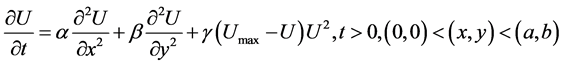 (1)
(1)
where: U is a temperatureα and β are diffusion parameters in direction of x and y, respectivelyγ is reaction parametera and b are plate dimensions in direction of x and y, respectivelyUmax is a maximum temperature of the system.
Along the external boundaries, the temperatures can be described as:
 (2-a)
(2-a)
 (2-b)
(2-b)
 (2-c)
(2-c)
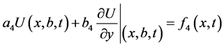 (2-d)
(2-d)
where  are known functions.
Then initial temperature may be described as:
 (3)
(3)
where  is a known function.
2.1. Numerical Procedure Using First Method (RK4)
The main strategy is to employ DQM to reduce the problem to a system of ordinary differential equations then to apply RK4 to solve the reduced system as follows:
1) Discretize the spatial domain using Chebyshev-Gauss-Lobatto grid points [12], such as:
 (4-a)
(4-a)
 (4-b)
(4-b)
2) Apply the method of differential quadrature in terms of nodal temperature, such that:
 (5-a)
(5-a)
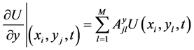 (5-b)
(5-b)
 (5-c)
(5-c)
 (5-d)
(5-d)
where ![]() and
and![]() ,
,  are the first and second order weighting coefficients with respect to p [12].
3) On sustainable substitution from Equations (5) into (1), one can reduce the problem to the following system of ordinary differential equations as:

or simply
 (6)
(6)
where
 (7)
(7)
4) Update the temperature using RK4 such that [16]
 (8)
(8)
where
![]() , (9-a)
, (9-a)
 (9-b)
(9-b)
 (9-c)
(9-c)
 , (9-d)
where 
2.2. Numerical Procedure Using Second Method (Implicit Euler)
The main strategy is to apply perturbation method of second order [17,18] then applying DQ discretization to reduce the problem to a system of ordinary differential equations then applying implicit Euler method to transform the previous system to a system of linear algebraic equations as follows:
1) We can solve
 (10)
(10)
subjected to the prescribed to boundary and initial conditions in Equations (2) and (3), assuming
 (11)
(11)
where  are unknowns functions and
  is a perturbation parameter.
The following condition is tested to ensure the convergence condition [19] in previous series in Equation (11).
 (12)
(12)
2) On sustainable substitution from Equation (11) into (10), one can reduce the problem to the following equation.
 (13)
(13)
3) Applying zero order perturbation method such that,
 (14)
(14)
Subjected to boundary and initial conditions in Equations (2) and (3), where differential quadrature method and implicit method are used to reduce Equation (14) to a system of linear algebraic equations such thatBy substitution of Equation (5) into (14) result that,
 (15)
(15)
 (16)
(16)
 (17)
(17)
4) First order perturbation method is applied such that,
 (18)
(18)
Subjected to the same boundary and initial conditions in Equations (2) and (3), reduced to the following algebraic system in equations
 (20)
(20)
 (21)
(21)
5) Also second order perturbation method is applied such that,
 (22)
(22)
Subjected to the same boundary and initial conditions in Equations (2) and (3), reduced to the following algebraic system
 (23)
(23)
 (24)
(24)
Finally, the series solution can be written as
 (25)
(25)
We carry on previous procedure until the specified time is reached.
3. Results and Discussions for One Dimension Analysis
To ensure the accuracy of the proposed numerical techniques, the thermal wave propagating model is solved using presented methods and compared with the available analytical solution [14,20].
Consider a one-dimensional problem of thermal wave propagation along x-direction as:
 .
.
While
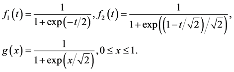 (26)
(26)
The exact solution for such problem can be obtained as [20]:
 (27)
(27)
To validate the accuracy of numerical results, the following errors [16] are computed,
 (28-a)
 (28-b)
3.1. Numerical Results of First Method (RK4)
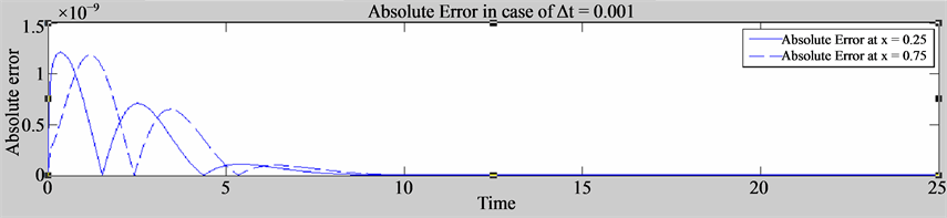
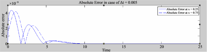
For the numerical computation, the time domain is limited to ![]() and N = 7. The efficiency of presented techniques is tested by CPU time required when the computation reaches to t = 20 s. Two time step sizes of 0.001 and 0.005 are used for layer marching in the time direction. The numerical results of these two cases are listed respectively in Tables 1 and 2. From these two tables, it can be seen that RK4 method can achieve high accuracy at very small step size at Δt = 0.001 with
and N = 7. The efficiency of presented techniques is tested by CPU time required when the computation reaches to t = 20 s. Two time step sizes of 0.001 and 0.005 are used for layer marching in the time direction. The numerical results of these two cases are listed respectively in Tables 1 and 2. From these two tables, it can be seen that RK4 method can achieve high accuracy at very small step size at Δt = 0.001 with  and at Δt = 0.005 with
 . Moreover, as shown in Figure 1, as Δt increased slightly to 0.00515 the stability condition will not achieved and the oscillation will occurs in the period
![]() . On the other hand the efficiency is very small as the CPU time required to reach t = 20 s is much larger.
. On the other hand the efficiency is very small as the CPU time required to reach t = 20 s is much larger.

Table 1. R.M.S., absolute errors, time steps and CPU times given by 4-stage Runge-Kutta at Δt = 0.001.
Table 2. R.M.S., absolute errors, time steps and CPU times given by 4-stage Runge-Kutta at Δt = 0.005.
3.2. Numerical Results of Second Method (Implicit Euler)
In the obtained results the advantage of using an implicit scheme has been observed. Stability problems are not encountered due to the use of implicit time integration step and larger time increments can be used, e.g. for t = 30, ![]() can be taken. Table 3 shows the maximum absolute errors and root mean square of errors for a fixed time (t = 30.0) for various numbers of grid points. The accuracies by using N = 8, 11 are almost the same and there is a drop for N = 15. From the table, DQM is observed to give very good accuracy with a small number of grid points. For N = 15, the drop of accuracy is due to the ill-conditioned Vandermonde-system obtained after the DQM discretization, which is the known nature of DQM for large N [15]. Tables 4-6 give the comparison of the DQM solution with the exact solution in terms of maximum absolute error and root mean square of errors for small time levels and for the times tending to steady-state, respectively. The computations are carried out with N = 11 and it is seen to be enough to obtain the solution with five digits accuracy at steady-state. Moreover, Figure 2 shows the absolute error at different times and locations. Also convergence condition in Equation (12) is tested achieving higher accuracy at second order perturbation method as shown in Figure 3.
can be taken. Table 3 shows the maximum absolute errors and root mean square of errors for a fixed time (t = 30.0) for various numbers of grid points. The accuracies by using N = 8, 11 are almost the same and there is a drop for N = 15. From the table, DQM is observed to give very good accuracy with a small number of grid points. For N = 15, the drop of accuracy is due to the ill-conditioned Vandermonde-system obtained after the DQM discretization, which is the known nature of DQM for large N [15]. Tables 4-6 give the comparison of the DQM solution with the exact solution in terms of maximum absolute error and root mean square of errors for small time levels and for the times tending to steady-state, respectively. The computations are carried out with N = 11 and it is seen to be enough to obtain the solution with five digits accuracy at steady-state. Moreover, Figure 2 shows the absolute error at different times and locations. Also convergence condition in Equation (12) is tested achieving higher accuracy at second order perturbation method as shown in Figure 3.
4. Results and Discussions for Two Dimensions Analysis
Consider also a simple two dimensional problem with

 and
and

To show the effect of oscillation on figure we graph the absolute error in range 10 ≤ t ≤ 11
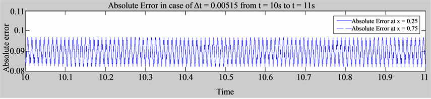
Figure 1. Absolute errors at different times and locations.
Table 3. R.M.S., absolute errors and CPU times given by implicit euler at Δt = 3.
Table 4. R.M.S., absolute errors and CPU times given by implicit euler at Δt = t.
Table 5. R.M.S., absolute errors and CPU times given implicit euler at Δt = 2.
Table 6. R.M.S., absolute errors and CPU times given by implicit euler at Δt = 4.
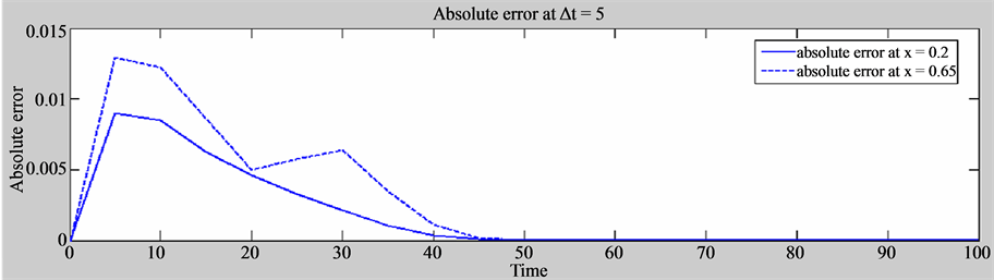
Figure 2. Absolute errors at different times and locations.
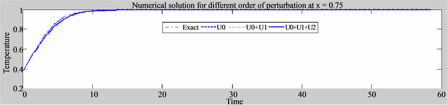
Figure 3. Satisfying convergence conditions.

which can be solved exactly as [21]: . The design of the numerical scheme is extended to two dimensions.
Table 7 shows that for , the obtained results agree with the analytical ones [21] in both methods. Also Figure 4 shows that absolute error for the hybrid method absolute error <0.01, and for implicit Euler, the absolute error
 .
.
5. Conclusion
Throughout this study, thermal wave propagation model which is the type of reaction-diffusion equations is solved by using DQM for space discretization and two different time-integration schemes. Moreover, one can use a small number of discretization points, which lead to higher accuracy. Also for the nonlinear wave equation, the use of DQM with non-uniform grid discretization increases the accuracy and stability of solution. The resulting system of ordinary differential equations is solved by using two different time integration schemes in order
Table 7 . Root mean square of errors for two dimensional thermal wave propagation at Δt = 0.01, N = 5, M = 4.
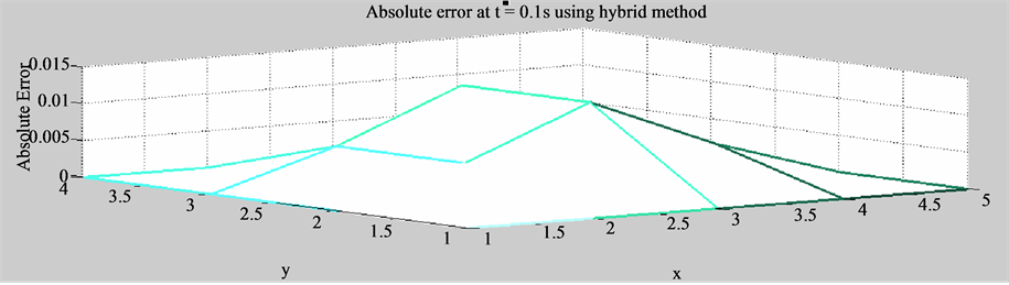
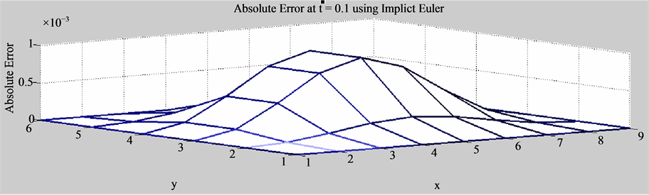
Figure 4. Absolute error at t = 0.1 s and different locations of x, y.
to make comparison between two methods and detect which of them is better. The numerical results obtained in this paper ensure that the problems have small desired time to reach it. Thus they have very small step size which is preferred and use RK4 to solve the system of ordinary differential equations in order to decrease the computational time. On the other hand, the problems which have high desired time to reach it, thus have large incremental time (stiff problems) which are preferred and use implicit Euler with perturbation method to solve the system of ordinary differential equations.
REFERENCES
- J. Opsal, A. Rosencwaig and D. L. Willenborg, “Thermal-Wave Detection and Thin-Film Thickness Measurements with Laser Beam Deflection,” Applied Optics, Vol. 22, No. 20, 1983, pp. 3169-3176. http://dx.doi.org/10.1364/AO.22.003169
- Z. Y. Yan, “Generalized Method and Its Application in the Higher-Order Nonlinear Schrodinger Equation in Nonlinear Optical Fibres,” Chaos Solitons and Fractals, Vol. 16, No. 5, 2003, pp. 759-766. http://dx.doi.org/10.1016/S0960-0779(02)00435-6
- J. Mei, H. Zhang and D. Jiang, “New Exact Solutions for a Reaction-Diffusion Equation and a Quasi-Camassa Holm Equation,” Applied Mathematics E-Notes, Vol. 4, 2004, pp. 85-91.
- E. S. Fahmy and H. A. Abdusalam, “Exact Solutions for Some Reaction Diffusion Systems with Nonlinear Reaction Polynomial Terms,” Applied Mathematical Sciences, Vol. 3, No. 11, 2009, pp. 533-540.
- M. S. H. Chowdhury and I. Hashim, “Analytical Solution for Cauchy Reaction-Diffusion Problems by Homotopy Perturbation Method,” Sains Malaysiana, Vol. 39, No. 3, 2010, pp. 495-504.
- S. Puri and K. Wiese, “Perturbative Linearization of Reaction-Diffusion Equations” Journal of Physics A: Mathematical and General, Vol. 36, No. 8, 2003, pp. 2043-2054. http://dx.doi.org/10.1088/0305-4470/36/8/303
- L. D. Ropp, N. J. Shadid and C. C. Ober, “Studies of the Accuracy of Time Integration Methods for Reaction-Diffusion Equations,” Journal of Computational Physics, Vol. 194, No. 2, 2004, pp. 544-574. http://dx.doi.org/10.1016/j.jcp.2003.08.033
- R. G. Marcus, “Finite-Difference Schemes for Reaction-Diffusion Equations Modeling Predator-Prey Interactions in MATLAB,” Bulletin of Mathematical Biology, Vol. 69, No. 3, 2007, pp. 931-956. http://dx.doi.org/10.1007/s11538-006-9062-3
- B. Liu, M. B. Allen, H. Kojouharov, B. Chen, et al., “Finite-Element Solution of Reaction-Diffusion Equations with Advection” Computational Mechanics, 1996, pp. 3-12.
- X. Christos and L. Oberbroeckling, “On the Finite Element Approximation of Systems of Reaction-Diffusion Equations by p/hp Methods,” Global Science, Vol. 28, No. 3, 2010, pp. 386-400.
- G. Meral and M. S. Tezer, “Solution of Nonlinear Reaction-Diffusion Equation by Using Dual Reciprocity Boundary Element Method with Finite Difference or Least Squares Method,” Advances in Boundary Element Techniques, Vol. 3, 2008, pp. 317- 322.
- C. Shu, “Differential Quadrature and Its Application in Engineering,” Springer Verlag, London, 2000. http://dx.doi.org/10.1007/978-1-4471-0407-0
- T. Y. Wu and G. R. Liu, “A Differential Quadrature as a Numerical Method to Solve Differential Equations,” Computational Mechanics, Vol. 24, No. 3, 1999, pp. 197-205. http://dx.doi.org/10.1007/s004660050452
- V. Kajal, “Numerical Solutions of Some Reaction-Diffusion Equations by Differential Quadrature Method,” International Journal of Applied Mathematics and Mechanics, Vol. 6, No. 14, 2010, pp. 68-80.
- G. Meral, “Solution of Density Dependent Nonlinear Reaction-Diffusion Equation Using Differential Quadrature Method,” World Academy of Science, Engineering and Technology, Vol. 41, 2010, pp. 1178-1183.
- W. Y. Yang, W. Cao, T. Chung, J. Morris, et al., “Applied Numerical Methods Using Matlab,” John Wiley & Sons, Hoboken, 2005. http://dx.doi.org/10.1002/0471705195
- J. S. Nadjafi and A. Ghorbani, “He’s Homotopy Perturbation Method: An Effective Tool for Solving Nonlinear Integral and Integro-Differential Equations,” Computers and Mathematics with Applications, Vol. 58, No. 11-12, 2009, pp. 2379-2390. http://dx.doi.org/10.1016/j.camwa.2009.03.032
- H. S. Prasad and Y. N. Reddy, “Numerical Solution of Singularly Perturbed Differential-Difference Equations with Small Shifts of Mixed Type by Differential Quadrature Method,” American Journal of Computational and Applied Mathematics, Vol. 2, No. 1, 2012, pp. 46-52. http://dx.doi.org/10.5923/j.ajcam.20120201.09
- J. P. Hambleton and S. W. Sloan, “A Perturbation Method for Optimization of Rigid Block Mechanisms in the Kinematic Method of Limit Analysis,” Computers and Geotechnics, Vol. 48, 2013, pp. 260-271. http://dx.doi.org/10.1016/j.compgeo.2012.07.012
- M. Bastani and D. K. Salkuyeh, “A Highly Accurate Method to Solve Fisher’s Equation,” Indian Academy of Sciences, Vol. 78, No. 3, 2012, pp. 335-346.
- E. Kreyszig, “Advanced Engineering Mathematics,” John Wiley & Sons, Columbus, 2006.