Applied Mathematics
Vol.4 No.1A(2013), Article ID:27487,10 pages DOI:10.4236/am.2013.41A027
Application of Laplace Transform for a Gas-Liquid-Solid Trickle Bed Reactor by Using the Tracer Technique
Environmental and Energetic Technology Laboratory, Polytechnic School (UPE), Recife, Brazil
Email: jornandesdias@poli.br
Received July 11, 2012; revised September 8, 2012; accepted September 15, 2012
Keywords: Trickle Bed Reactor; Experimental Setup; Mathematical Model; Laplace Transform; Dynamic; Hydrodynamic Parameters
ABSTRACT
Experimental evaluation and dynamic modelling were presented for a liquid flow (H2O + NaOH tracer) on solid particles in a trickle bed reactor. One-dimensional dynamic mathematical model has been described to study the gas-liquid-solid process in which the liquid phase with the NaOH tracer is treated as a continuum. The physical model has been analyzed, including the formulation of initial and boundary conditions and the description of the solution methodology. An experimental setup to measure the concentrations of the NaOH tracer has been performed. The concentration measurements of this NaOH tracer have been performed in a fixed be reactor on trickling flow of the liquid phase for a range of operating conditions. The axial dispersion (Dax) of the liquid phase, liquid-solid mass transfer (kLS) coefficient and partial wetting efficiency (fe) were chosen as the hydrodynamic parameters of the proposed mathematical model. Such parameters have been optimized with experimental measurents of the NaOH tracer at the exit of the trickle-bed reactor. The optimized parameters (Dax, kLS and fe) were calculated simultaneously by using the theoretical model with minimization of the objective function. Results of the proposed mathematical model have been presented and compared as of the two experimental cases. These hydrodynamic parameters were fitted by means of the empirical correlations.
1. Introduction
Mathematical models of TBRs represent an ancillary tool for minimizing the experimental efforts required to developing this important equipment in industrial plants. Experiment and prototype development are the main requirements for accurate engineering design in any Industrial process. However, mathematical modelling and numerical simulation are in continuous development, contributing in a growing form for the better understanding of processes and physical phenomena, and in which for design. generally, mathematical models require experiment in order to be validated and the required experiments involve complex measurements of difficult accomplishment. Therefore, mathematical modelling also represents an incentive for the development of new experimental methods.
Trickle-bed reactors (TBRs) were defined as fixed beds of catalyst particles in connection with the co-current downward flows of gas and liquid phases at low superficial velocities. These reactors assume greater importance among the there-phase gas-liquid-solid reaction systems encountered in industrial processes. TBRs are extensively used in many process industries. These reactors are widely employed in petroleum refineries for hydrotreating, hydrodemetalization and hydrocracking applications. On the other hand, they also are widely used for carrying out a variety of processes such as petrochemical, chemical, biochemical and waste treatment. There are many works in the literature to model and describe the behaviour of processes of those TBRs. The behaviour to many of those works can be studied applying mathematical modelling.
Various flow regimes exist in a TBR depending on the liquid and gas mass flow rates, the properties of the fluids and the geometrical characteristics of the packed bed [1]. A fundamental understanding of the hydrodynamics of TBRs is indispensable in their design, scale-up and performance. The hydrodynamics are affected differently in each flow regime. The basic hydrodynamics parameters for the design are scale-up and operation, the pressure gradient and liquid saturation. The pressure gradient is related for the mechanical energy dissipation due to the two-phase flow through the fixed bed of solid particles. The liquid saturation which partially occupies the void volume of the packed bed is related to other important hydrodynamics parameters as the pressure gradient, the external wetting of the catalyst particles, the mean residence time of the liquid phase in the reactor and the heat and mass transfer phenomena [2,3].
There are various mathematical models of completely or partially wetted catalyst particles which may exist in TBRs. Those models are based on many assumptions and they are forced to using simplifications to solve the complex equation systems. Mathematical models of TBRs may involve the mechanisms of forced convection, axial dispersion, interphase heat and mass transfers, intraparticle diffusion, adsorption, and chemical reaction [4,5].
The present work has like objectives to optimize the axial dispersion (Dax) of the liquid phase, liquid-solid mass transfer (kLS) coefficient, and partial wetting efficiency (fe) by using different set of experiments carried out in one laboratory scale TBR. Validating by comparson with three experimental cases the proposed mathematical. Developing the empirical correlations for the parameters (Dax, kLS and fe) by using the experimental values of these parameters.
2. Mathematical Modelling
In this work, the mathematical modelling has been based on the liquid-solid model which treats the liquid phase (H2O + NaOH tracer) as a continuum on a fixed bed of solid particles. An one-dimensional dynamic mathematical model has been adopted where the axial dispersion, liquid-solid mass transfer, partial wetting, and reaction phenomena are present. This model was presented for the liquid phase by using the NaOH as a tracer and it is restricted to the following assumptions: 1) Isothermal system; 2) All flow rates are constant through the reactor; 3) The intraparticle diffusion resistance has been neglected; 4) In any position of the reactor the chemical reaction rate is equal to the liquid-solid mass transfer rate at the particle surface.
• Mass balance for the liquid;
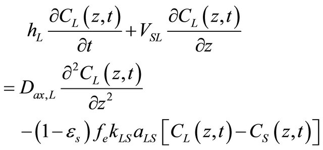 (1)
(1)
• The initial and boundary conditions for the Equation (1) are given as:
 ; for all z (2)
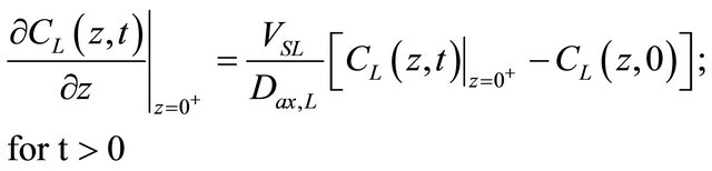 (3)
(3)
 (4)
(4)
The equality of mass transfer and reaction rates were expressed by the following equations:
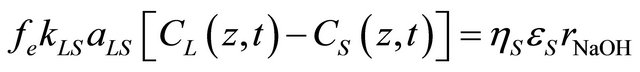 (5)
(5)
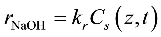
The kinetic model for the reaction was based on a first-order reaction according to the equation below [6]:
 (6)
(6)
Where rNaOH is the consumption rate of the reactant, Cs(z,t) is the reactant concentration at the surface of the solid phase, and kr is the reaction rate constant of the first-order reaction. Combining Equations (5) and (6), the rate of mass transfer is equal the rate of reaction at the surface of the solid phase as:
 (7)
(7)
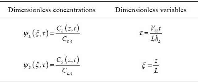
Equations (1)-(4), and (7) can be analyzed with dimensionless variable terms, see Table 1.
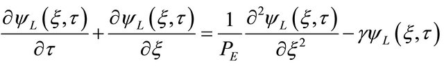
Writing Equations (1)-(4), and (7) in dimensionless forms:
 (8)
(8)
 ; for all
  (9)
(9)
 (10)
(10)
 (11)
(11)
 (12)
(12)
Equations (8)-(12) include the following dimensionless parameters:
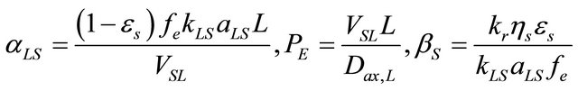 (13)
(13)
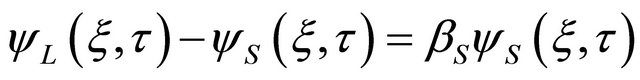
The dimensionless concentration, ΨS (ξ, τ), was isolated of the Equation (12) and it has been introduced in the Equation (8) reducing it to:
Table 1. Summary of dimensionless variables.
 (14)
(14)
where: 
3. Solution in the Laplace Domain
Applications of the Laplace Transform (LT) on dynamic transport problems in three-phase trickle bed reactors with tracer (liquid or gaseous) are very popular in chemical engineering. Laplace transformations are powerful means by solving linear differential equations. Although the potency of complex analysis, the analytical Laplace inversion often fails, thus necessitating numeral inversion. However, the LT technique with respect to time has been applied on the partial differential Equation (14) and its initial and boundary conditions given by Equations (9)- (11), as presented below:
• The Equation (14) in the Laplace domain;
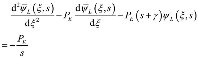 (15)
(15)
where the overhead sign (-) indicates the LT, and s is the LT parameters.
• The initial and boundary conditions in the Laplace domain;
 (16)
(16)
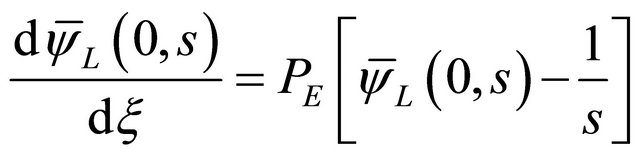 (17)
(17)
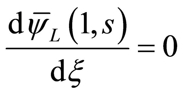 (18)
(18)
The Equation (15) is known as one second-order nonhomogeneous ordinary differential equation. Its general solution is the sum of the general solution of its corresponding homogeneous ordinary differential equation and a particular solution, that is:
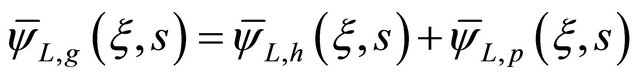 (19)
(19)
where  is the solution for the second-order homogeneous ordinary differential equation and
  is the particular solution.
The first step is to find the solution from the secondorder homogeneous ordinary differential equation, as shown below:
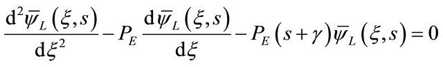 (20)
(20)
The characteristic equation for the Equation (20) is given as:
 (21)
(21)
So the roots from the Equation (21) are presented by:
 (22)
(22)
 (23)
(23)
The general solution of the corresponding homogeneous ordinary differential equation from the Equation (20) is obtained as:
 (24)
(24)
The Equation (24) can be written in the following form:
 (25)
(25)
where b1 and b2(s) are defined below, respectively.
 (26)
(26)
Using concepts of hyperbolic functions according to the following relationships below:
 (27)
(27)
 (28)
(28)
However, the Equation (28) was written as:
 (29)
(29)
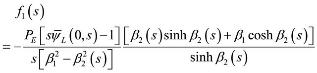
where f1(s) and f2(s) are expressed by:
 (30)
(30)
The second step is obtained the particular solution from the Equation (15). The  term from the Equation (15) was given as one constant value. For simplicity, we consider here the particular solution as:
 (31)
(31)
The above Equation (31) was constructed by using the method of undetermined coefficients. The result from the Equation (31) was usually obtained according to the following expression for the .
.
 (32)
(32)
The general solution has been presented by the Equation (19), in which  and
and  were attributed according to the result below:
 (33)
(33)
where f1(s) and f2(s) are two arbitrary integration constants. By using the boundary conditions from Equations (17) and (18) to the general solution, Equation (33). It was led to the algebraic equations needed to find the arbitrary integration constants f1(s) and f2(s) in terms of known parameters. The expressions for these two constants have been found here as:
 (34)
(34)
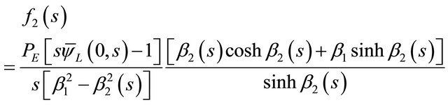 (35)
(35)
For ξ = 1 it was possible to obtain the concentration of the tracer at the exit of the fixed bed. However, the expressions of Equations (34) and (35) were introduced in Equation (33) to obtain the general solution of the tracer concentration in liquid phase according to as follow [7].
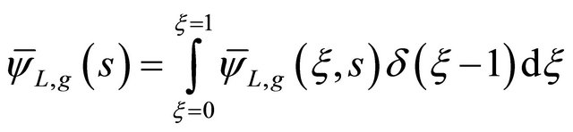 (36)
(36)
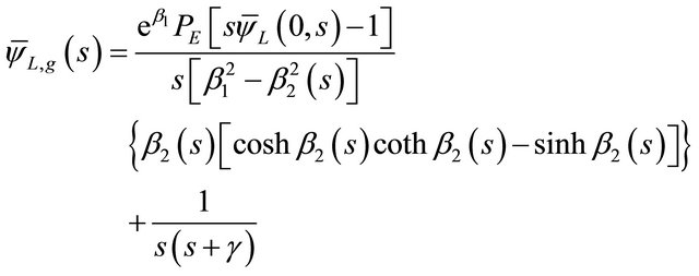 (37)
(37)
The analytical inverse Laplace transformation from the Equation (39) is a very complicated mathematical problem. So it, the Equation (39) will be used to obtain the concentration of the tracer at the exit of the trickle-bed reactor by numerical inversion using the numerical fast Fourier transform (NFFT) technique. By using the NFFT technique for a disturbance of the type positive step can be obtained from the following expression [8,9].
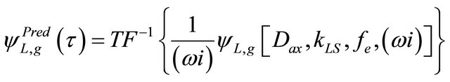 (38)
(38)
where the Laplace variable (s) was changed by (wi) in the Fourier domain.
4. Experimental Setup
The experiments were realized in a three-phase trickle bed reactor, in which consists of a fixed bed with 0.22 m height and 0.030 m inner diameter with catalytic particles contacted by a cocurrent gas-liquid downward flow carrying the NaOH tracer in the liquid phase. The experiments have been performed on conditions where the volumetric flow rates for the gas and liquid phases were maintained at such a level to guarantee the low interaction regime in 7.068 × 10⁻⁸ m3∙s−1 to 2.122 × 10⁻⁶ m3∙s−1 liquid flowing (QL) and in 6.437 × 10⁻⁶ m3∙s−1 to 3.181 × 10⁻⁴ m3∙s−1 gas flowing (QG) in a pilot plant trickle be reactors [10-12].
Continuous analysis for the NaOH tracer, in a 10 mol∙m−3 concentration, was made by using HPLC/UVCG 480 C at the exit of the fixed bed. Results have been expressed in term of the NaOH tracer concentrations versus time (positive step).
Continuous analysis for the NaOH tracer, in a 10 mol∙m−3 concentration, was made by using HPLC/UVCG 480C at the exit of the fixed bed. Results have been expressed in term of the NaOH tracer concentrations versus time (positive step).
• Analysis for the positive-step experimental results at the exit of the fixed bed;
• Comparison for the experimental results obtained at the exit of the bed with those results from the Equation (38) by using the minimization of the objective function [13], given by:
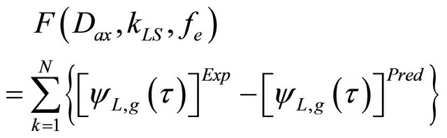 (39)
(39)
• Computation for the parameters (Dax, kLS, and fe) from the mathematical. The initial values for the parameters (Dax, kLS, and fe) were considered by means of the proposed empirical correlations in literature according to the Table 2;
Table 2. Empirical correlations for the obtainment of the Dax, kLS and fe, the initial values.
• 
• Optimizing the Dax, kLS, and fe parameters by means of the comparison between the experimental and theoretical results through the Equation (39).
5. Results and Discussion
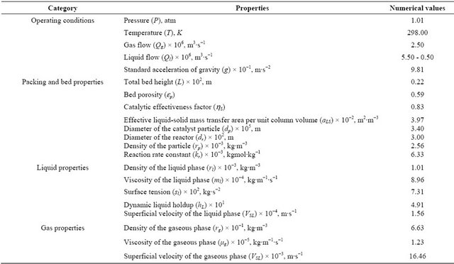
Various fixed parameters were used to calculate the concentrations of the NaOH reactive tracer as of the proposed mathematical model. These parameters are presented according to the Table 3. In this Table, it were shown the values for four categorical properties such as the operating conditions, packing and bed properties, liquid properties and gas properties.
Experiments were performed for a constant volumetric flow rate (QG = 2.500 × 10⁻⁶ m3∙s−1) of the gas phase and variable volumetric flow rate (QL = 5.500 × 10⁻⁶ m3∙s−1 to 0.500 × 10⁻⁶ m3∙s−1) of the liquid phase. Experimental procedures as well as results are presented in details in the tricking flow regime. Results obtained from the mathematical model were compared with such experimental sets. An objective function (F) has been calculated and presented. Values of the objective function indicate a very good fit between the proposed mathematical model and experimental results. The computation methodology to optimize the parameters (Dax, kLS and fe) involved numerical inversion in the Fourier domain followed by a minimization of the objective function [17, 18].
In the studied trickling flow regime, our experimental results for Dax, kLS and fe are well correlated by means of the following equations:
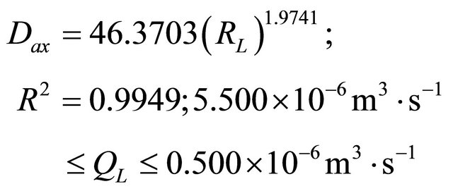 (40)
(40)
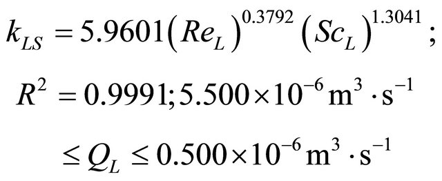 (41)
(41)
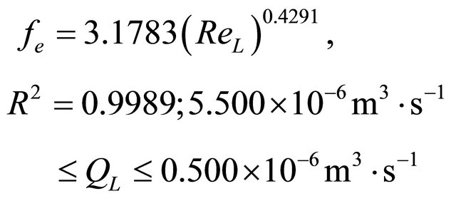 (42)
(42)
The parameters (Dax, kLS and fe) have been optimized as of the Equation (39) with their variable volumetric flow rates of the liquid phase. The parameter (Dax) of the liquid phase is varying from 3.585 × 10⁻⁶ m2∙s−1 to 1.057 × 10⁻⁶ m2∙s−1. As long as, the kLS parameter is changing from 2.298 × 10⁻⁶ m2∙s−1 to 0.123 × 10⁻⁶ m2∙s−1. On the other hand, FM parameter is differentiating from 0.681 to 0.459. The optimization for the parameters Dax, kLS and fe) have been performed by means of the minimization of the objective function. This objective function is varying 3.231 × 10⁻⁵ to 1.093 × 10⁻⁵, respectively.
Table 3. Summary of intervals of operating conditions for the particle-fluid.
The mean relative errors (MRE) between the predicted and experimental results for the Dax, kLS and fe parameters were computed as of the following equation:
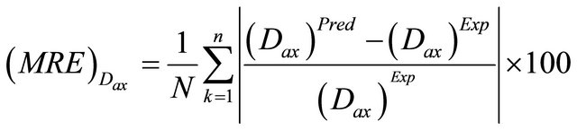 (43)
(43)
 (44)
(44)
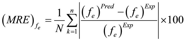 (45)
(45)
where (Dax)Pred, (kLS)Pred and (fe)Pred are calculated by means of Equations (40)-(42) above. On the other hand, (Dax)Exp, (kLS)Exp and (fe)Exp are obtained from the Equation (39) together with the experimental results.
Tables 4-6 show the experimental and theoretical results together with the mean relative errors for each parameter, respectively.
Table 4. Experimental and theoretical results for the (Dax)Exp and (Dax)Pred obtained by means of Equations (39) and (40) as well as the mean relative errors determined through the Equation (43).
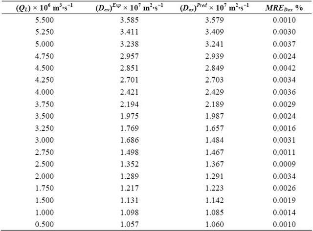
Table 5. Experimental and theoretical results for the (kLS)Exp and (kLS)Pred obtained by means of Equations (39) and (41) as well as the mean relative errors determined through the Equation (44).
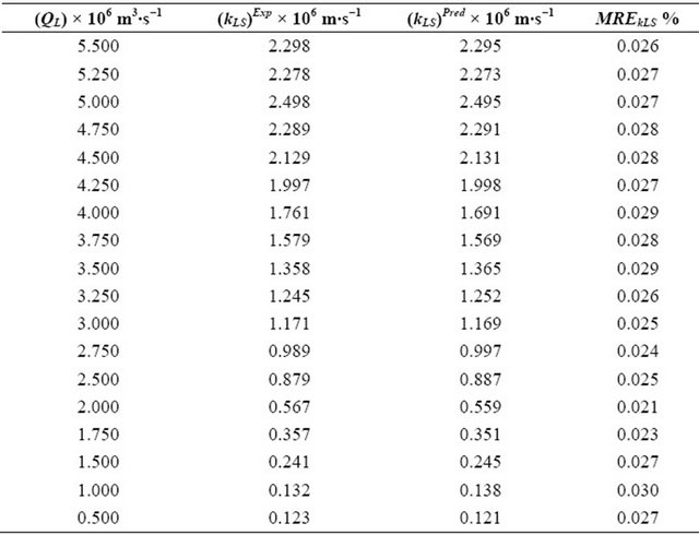
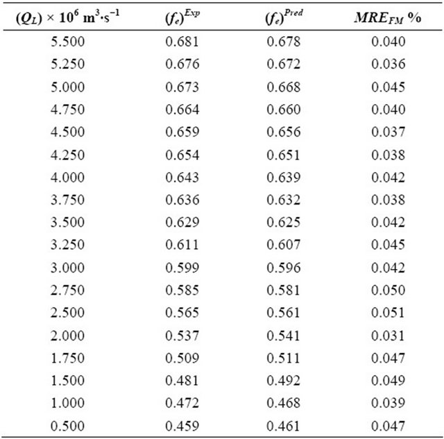
Table 6. Experimental and theoretical results for the (FM)Exp and (fe)Pred obtained by means of Equations (39) and (42) as well as the mean relative errors determined through the Equation (45).
The experimental results concerning the volumetric flow rates (QL = 1.750 × 10⁻⁶ m3∙s−1 and QL = 4.750 × 10⁻⁶ m3∙s−1) were used for the proposed mathematical model validation, but not considered to fit the parameters (Dax., kLS and fe). The validation process was established in comparison with the experimental and simulated results. The simulated results have been obtained by using the empirical correlations described by Equations (40)- (42) together with the numerical values presented in Table 3. These comparisons between the experimental and simulated results can be seen in Figures 1 and 2. In Figures 1 and 2, the simulated curves shown an excellent agreement in comparison with the experimental points. This is a good indication that there is no systematic discrepancy between model and experiments for the data set as a whole.
Figures 3-5 show the behavior for the Dax, kLS and fe parameters in comparison with the experimental and calculated results with the exception of the volumetric flow rates (QL = 1.750 × 10⁻⁶ m3∙s−1 and QL = 4.750 × 10⁻⁶ m3∙s−1). Results for the mean relative errors shown in Tables 4-6 indicate that there is no systematic discrepancy between experimental and calculated data.

Figure 1. Comparison between the experimental and simulated concentrations for the NaOH tracer at the exit of the fixed bed versus dimensionless time on the following conditions: 298 K, 1.01 bar, QG = 2.500 × 10⁻⁶ m3∙s−1 and QL = 1.750 × 10⁻⁶ m3∙s−1, Dax, L = 1.217 × 10⁻⁷ m2∙s−1, kLS = 0.357 × 10⁻⁶ m∙s−1 and fe = 0.509.
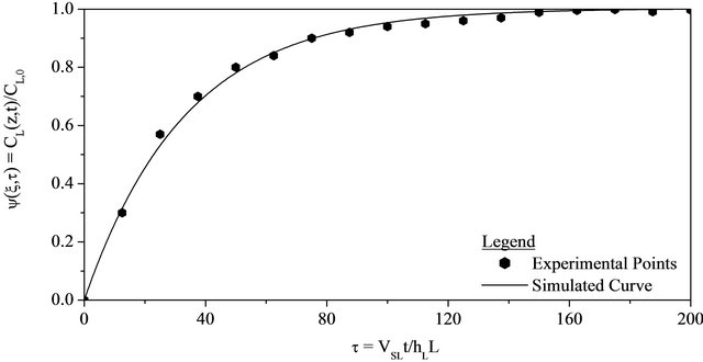
Figure 2. Comparison between the experimental and simulated concentrations for the NaOH tracer at the exit of the fixed bed versus dimensionless time on the following conditions: 298 K, 1.01 bar, QG = 2.500 × 10⁻⁶ m3∙s−1 and QL = 4.750 × 10⁻⁶ m3∙s−1, Dax, L = 2.957 × 10⁻⁷ m2∙s−1, kLS = 2.289 × 10⁻⁶ m∙s−1 and fe = 0.664.
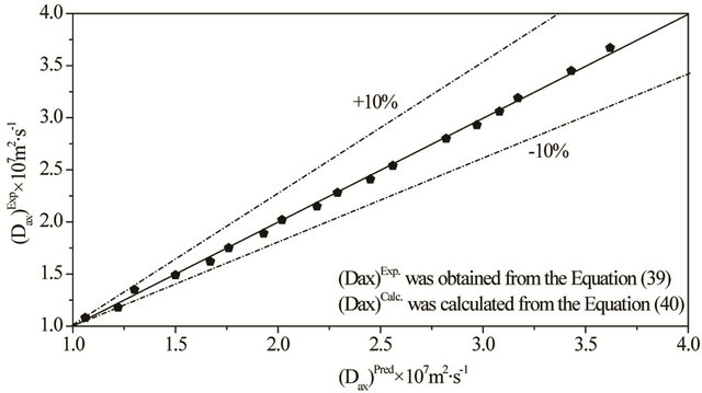
Figure 3. Parity (Dax)Exp versus (Dax)Pred for the system N2/H2O-NaOH/activated carbon operating in the low interaction regime. Conditions: 298 K, 1.01 bar QG = 2.500 × 10⁻⁶ m3∙s−1, QL = 5.500 × 10⁻⁶ m3∙s−1 to 0.500 × 10⁻⁶ m3∙s−1.

Figure 4. Parity (kLS)Exp versus (kLS)Pred for the system N2/H2O-NaOH/activated carbon operating in the low interaction regime. Conditions: 298 K, 1.01 bar QG = 2.500 × 10⁻⁶ m3∙s−1, QL = 5.500 × 10⁻⁶ m3∙s−1 to 0.500 × 10⁻⁶ m3∙s−1.
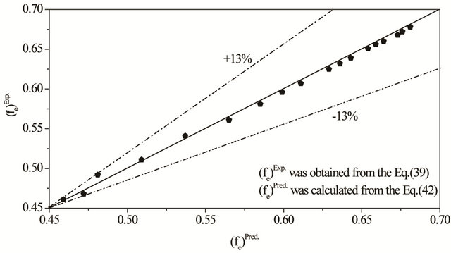
Figure 5. (fe)Exp versus (fe)Pred for the system N2/H2O-NaOH/activated carbon operating in the low interaction regime. Conditions: 298 K, 1.01 bar QG = 2.500 × 10⁻⁶ m3∙s−1, QL = 5.500 × 10⁻⁶ m3∙s−1 to 0.500 × 10⁻⁶ m3∙s−1.
6. Conclusion
Based on the experimental and modeling studies of the liquid phase in a low interaction system, the following results were obtained: 1) The estimation of the parameters Dax, kLS and fe; 2) The validation of the model and 3) The analysis of the behavior of the axial dispersion coefficient, liquid-solid mass transfer coefficient and Partial wetting efficiency by new forms of empirical correlationssee Equations (40)-(42). The final values of the parameters were obtained with values of the objective function, F = 3.231 × 10⁻⁵ to 1.093 × 10⁻⁵. Thus, the range of the optimized values of the parameters by fitting between the theoretical and experimental response were given as: Dax = 3.585 × 10⁻⁷ m2∙s−1 to 1.057 × 10⁻⁶ m2∙s−1, kLS = 2.298 × 10⁻⁶ m∙s−1 to 0.123 × 10⁻⁶ m∙s−1 and fe = 0.681 to 0.459.
6. Acknowledgements
The authors would like to thank CNPq (Conselho nacional de Desenvolvimento e Tecnológico) for financial support (process 483541/07-9).
REFERENCES
- J. C. Charpentier and M. Favier, “Some Liquid Holdup Experimental Data in Trickle Bed Reactors for Foaming and Non-Foaming Hydrocarbons,” Aiche Journal, Vol. 21, No. 6, 1975, pp. 1213-1221. doi:10.1002/aic.690210626
- V. Specchia and G. Baldi, “Pressure Drop and Liquid Holdup for Two Phase Cocurrent Flow in Packed Beds,” Chemical Engineering Science, Vol. 32, No. 5, 1977, pp. 515-523. doi:10.1016/0009-2509(77)87008-5
- A. Burghardt, B. Grazyna, J. Miczylaw and A. Kolodziej, “Hydrodynamics and Mass Transfer in a Three-Phase Fixed Bed Reactor with Concurrent Gas-Liquid Downflow,” Chemical Engineering Journal, Vol. 28, 1995, pp. 83-99.
- I. Iliuta, S. C. Bildea, M. C. Iliuta and F. Larachi, “Analysis of Trickle Bed and Packed Bubble Column Bioreactors for Combined Carbon Oxidation and Nitrification,” Brazilian Journal of Chemical Engineering, Vol. 19, No. 3 2002, pp. 69-87.
- M. A. Latifi, A. Naderifar and N. Midoux, “Experimental Investigation of the Liquid-Solid Mass Transfer at the Wall of Trickle Bed—Influence of Schmidt Number,” Chemical Engineering Science, Vol. 52, No. 21-22, 1997, pp. 4005-4011. doi:10.1016/S0009-2509(97)00243-1
- A. J. Colombo, G. Baldi and S. Sicardi, “Solid-Liquid Contacting Effectiveness in Trickle-Bed Reactors,” Chemical Engineering Science, Vol. 31, No. 12, 1976, pp. 1101-1108. doi:10.1016/0009-2509(76)85019-1
- J. D. Silva, F. R. A. Lima, C. A. M. Abreu and A Knoechelmann, “Experimental Analysis and Dynamic Modeling of the Mass Transfer Processes for a Fixed Bed Three-Phase Reactor in Trickle Bed Regime,” Brazilian Journal of Chemical Engineering, Vol. 20, No. 4, 2003, pp. 375-390. doi:10.1590/S0104-66322003000400005
- J. D. Silva, “Dynamic Evaluation for Liquid Tracer in a Trickle Bed Reactor,” Journal of the Brazilian Society of Mechanical Sciences and Engineering, Vol. 33, No. 3, 2011, pp. 277-272. doi:10.1590/S1678-58782011000300002
- P. A. Ramachandran and R. B. Chaudhari, “Three Phase Catalytic Reactors,” Gordon and Breach Science Publishers, New York, 1983, pp. 200-251.
- J. D. Silva, “Computation of Axial Dispersion and Overall Liquid Solid Mass Coeffients for a Trickle-Bed Reactor by Using the Tracer Technique”, 21st Brazilian Congress of Mechanical Engineering, 24-28 October 2011, Natal, pp. 1-10.
- J. G. Rodrigo, L. Rosa and M. Quinta-Ferreira, “Turbulence Modelling of Multiphase Flow in High-Pressure Trickle Reactor,” Chemical Engineering Science, Vol. 64, No. 8, 2009, pp. 1806-1819. doi:10.1016/j.ces.2008.12.026
- F. Augier, A. Koudil, L. Muszynski and Q. Yanouri, “Numerical Approach to Predict Wetting and Catalyst Efficiencies Inside Trickle Bed Reactors,” Chemical Engineering Science, Vol. 65, No. 1, 2010, pp. 255-260. doi:10.1016/j.ces.2009.06.027
- P. Box, “A New Method of Constrained Optimization and a Comparison with Other Method,” Computer Journal, Vol. 8, No. 1, 1965, pp. 42-52. doi:10.1093/comjnl/8.1.42
- R. Lange, R. Gutsche and J. Hanika, “Forced Periodic Operation of a Trickle-Bed Reactor,” Chemical Engineering Science, Vol. 54, No. 13-14, 1999, pp. 2569-2573. doi:10.1016/S0009-2509(99)00004-4
- S. Fukushima and K. Kusaka, “Interfacial Area Boundary of Hydrodynamic Flow Region in Packed Column with Cocurrent Downward Flow,” Journal of Chemical Engineering of Japan, Vol. 10, No. 6, 1977, pp. 461-467. doi:10.1252/jcej.10.461
- A. Burghardt, A. S. Kolodziej and J. Zynski, “Experimental Studies of Liquid-Solid Wetting Efficiency in Trickle-Bed Cocurrent Reactors,” Chemical Engineering Journal, Vol. 28, 1990, pp. 35-49.
- A. Ayude, J. Cechini, M. Cassanello, O. Martínez and P. Haure, “Trickle Bed Reactors: Effect of Liquid Flow Modulation on Catalytic Activity,” Chemical Engineering Science, Vol. 63, No. 20, 2008, pp. 4969-4973. doi:10.1016/j.ces.2008.07.024
- G. Liu, X. Zhang, L. Wang, S. Zhang and Z. Mi, “Unsteady-State Operation of Trickle-Bed Reactor for Dicyclopentadiene Hydrogenation,” Chemical Engineering Science, Vol. 36, No. 20, 2008, pp. 4991-5001. doi:10.1016/j.ces.2008.03.008
Nomenclature
CL(z, t): Concentration of the liquid tracer in the liquid phase, kg∙m−3;
CS(z, t): Concentration of the liquid tracer in the external surface of solid, kg∙m−3;
aLS: Effective liquid-solid mass transfer area per unit column volume, m2∙m−3;
Dax: Axial dispersion coefficient for the liquid tracer in the liquid phase, m2∙s−1;
dP: Diameter of the catalyst particle, m;
dr: Diameter of the reactor, m;
F: Objective function;
fe: Wetting factor efficiency, dimensionless;
GaL: Galileo number,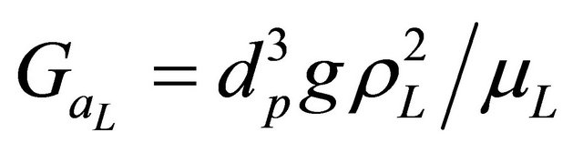 ;
;
hL: Dynamic liquid holdup, dimensionless;
i: Complex number ;
;
kr: Reaction constant, kgmol∙kg−1∙s−1;
L: Height of the catalyst bed, m;
PE: Peclet number,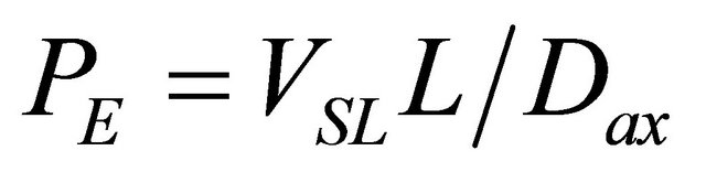 ;
;
ReL: Reynolds number,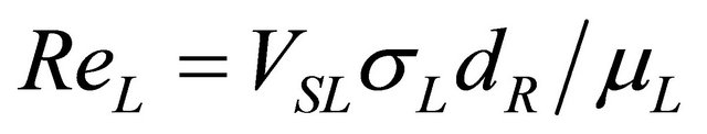 ;
;
ScL: Schmidt number, ;
;
t: Time, s;
VSL: Superficial velocity of the liquid phase, m∙s−1;
z: Axial distance of the catalytic reactor, m.
Greek Letters
αLS: Parameter defined in Equation (13), dimensionless;
bS: Parameter defined in Equation (15), dimensionless eP: internal porosity, dimensionless;
Ψi (ξ, τ): Dimensionless concentration of the tracer in liquid and solid, i = L, S;
hS: Catalytic effectiveness factor;
rL: Density of the liquid phase, kg∙m−3;
mL: Viscosity of the liquid phase, kg∙m−1∙s−1.