Applied Mathematics
Vol.3 No.9(2012), Article ID:22991,5 pages DOI:10.4236/am.2012.39142
Restricted Three-Body Problem in Different Coordinate Systems
—II-In Sidereal Spherical Coordinates System
1Department of Astronomy, Faculty of Science, King Abdulaziz University, Jeddah, KSA
2Department of Mathematics, Faculty of Science, King Abdulaziz University, Jeddah, KSA
Email: *sharaf_adel@hotmail.com, alshaary@hotmail.com
Received July 10, 2012; revised August 10, 2012; accepted August 17, 2012
Keywords: Spatial Restricted Circular Three Body Problem; Regularization; Coordinate Transformations
ABSTRACT
In this paper of the series, the equations of motion for the spatial circular restricted three-body problem in sidereal spherical coordinates system were established. Initial value procedure that can be used to compute both the spherical and Cartesian sidereal coordinates and velocities was also developed. The application of the procedure was illustrated by numerical example and graphical representations of the variations of the two sidereal coordinate systems.
1. Introduction
In a previous communication to this journal [1], hereafter referred to as Paper I we started our studies towards establishing new differential equations for the different forms of the three-body problem using some important coordinate systems. By this, we aims at obtaining differential equations (see [1] for details) which are: 1) Regular; 2) Suitable for the geometry to which they referred; 3) Producing slow variations in the coordinates during the orbital motion, a property which produces more stable numerical integration procedures. In Paper I, the equations of motion for spatial restricted circular three body problem in cylindrical coordinates system was established together with a computational algorithm that can be used to compute both the cylindrical and Cartesian coordinates and velocities. In the present paper, the equations of motion for the spatial circular restricted threebody problem in sidereal spherical coordinates system were established. Initial value procedure that can be used to compute both the spherical and Cartesian sidereal coordinates and velocities was also developed. The application of the procedure was illustrated by numerical example and graphical representations of the variations of the two sidereal coordinate systems.
2. Circular Restricted Three-Body Problem in Sidereal System
If two of the bodies, say m1 and m2 in the three-body problem move in circular, coplanar orbits about their common center of mass and the mass say m3 of the third body is too small to affect the motion of the other bodies, the problem of the motion of the third body is called the circular, restricted, three body problem. The two revolving bodies are called the primaries; their masses are arbitrary but have such internal mass distributions that they may be considered point masses.
The equations of motion of the third body in a dimensionless sidereal (inertial) coordinate  system with the mean motion
 , are [2]
 (1)
(1)
 (2)
(2)
 (3)
(3)
where  is given as
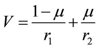 (4)
(4)
 denotes the mass of the smaller primary when the total mass of the primaries has been normalized to unity.
 (5)
(5)
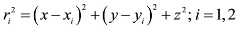
and  are the distances of the third body from the primaries which are located at
 ;
; , these coordinates are functions of the time t and are given as
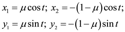 (6)
(6)
3. The Equations of Motion in Sidereal Spherical Coordinate System
Corresponding to the Cartesian sidereal coordinate system , the coordinate system related to the system
  by certain transformation, is also called sidereal coordinate system. In this respect the system
  of Equation (7) is called sidereal spherical coordinate system.
In what follows we shall establish, the differential equations for the spatial circular restricted three bodyproblem in sidereal spherical coordinate system.
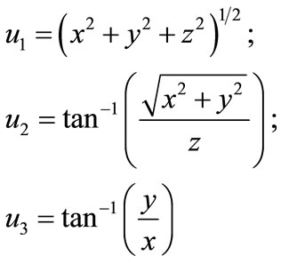
3.1. Coordinate and Velocity Transformations
 (7)
(7)
 (8.1)
(8.1)
 (8.2)
(8.2)
 (8.3)
(8.3)
where
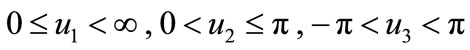 (9)
(9)
3.2. Inverse Transformations
From Equation (7) we have
 (10)
(10)
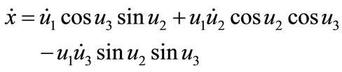
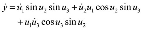
Differentiating the first and the third of Equation (10) and the third of Equation (7) with respect to the time t we get:
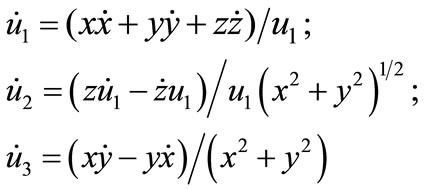 (11)
(11)
where  and
and  are given in terms of
  and
and  from the previous equations.
3.3. The Equations of Motion
The kinetic energy of a particle of unit mass in the spherical coordinate system is
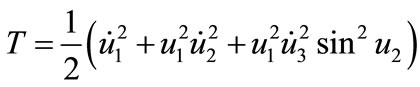 (12)
(12)
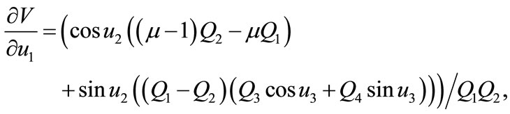
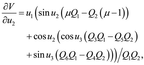
By using the transformation equations (Equations (7)), the gravitational potential V could be expressed in term of .
.
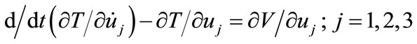
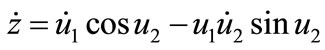
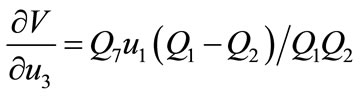
Consequently, we deduce for the equations of motion in sidereal spherical coordinate system, the forms
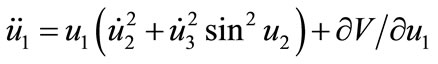 (13.1)
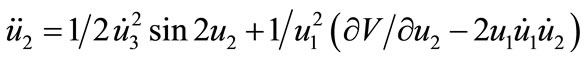 (13.2)
 (13.3)
where  are given as
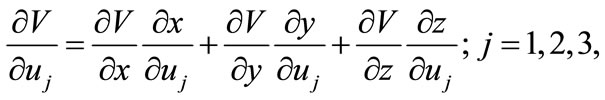 (14)
(14)
 ,
,  and
and ;
;  can be computed from Equation (7), while
 ,
,  and
and  can be computed from Equations (1)-(3), so we get
 where
where
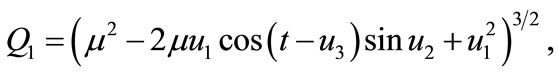
 ,
,
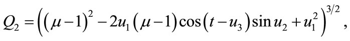
 ,
,
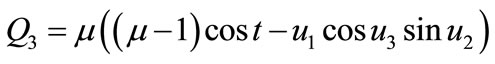
 ,
,
 .
.
4. Computational Development
4.1. Initial Value Procedure
In what follows, we shall establish a procedure that can be used to compute  (say) both:
1) The spherical sidereal coordinates and velocities , and 2) The Cartesian sidereal coordinates and velocities
 .
.
So, such procedure is a double usefulness computational algorithm, for which a differential solver can be used for the spherical sidereal six order system to obtain . While the Cartesian sidereal coordinates and velocities
  are obtained by the substitutions in the direct transformation formulae (Equations (7) and (8)), rather than solving the six order system of Equations (1), (2) and (3). By this way, great time can be saved.
This initial value procedure using sidereal spherical coordinate system will be described through its basic points, input, output and computational steps.
Input: 1)  at
at 2) the final time
3) 
Output: 1) 
2) 
Computational steps
1) Using the given values  at
at  and the inverse transformations to compute the initial values
 .
.
2) Using the partial derivatives  (functions of
 ) to construct the analytical forms of equations of motion as first order system.
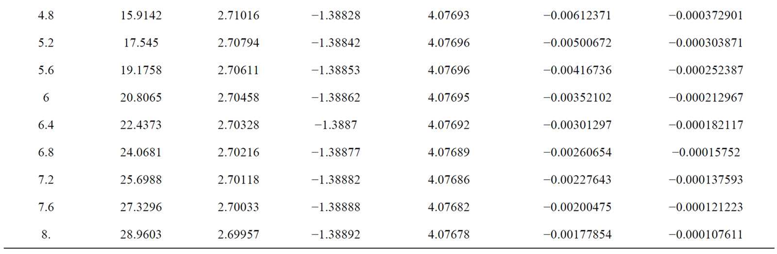
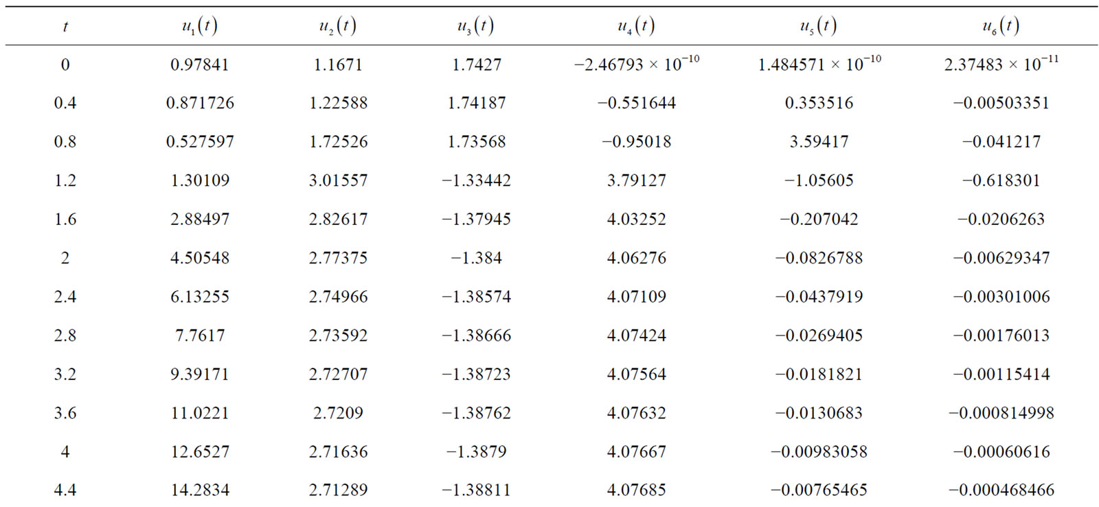
Table 1. The values of sidereal spherical coordinates and velocities.
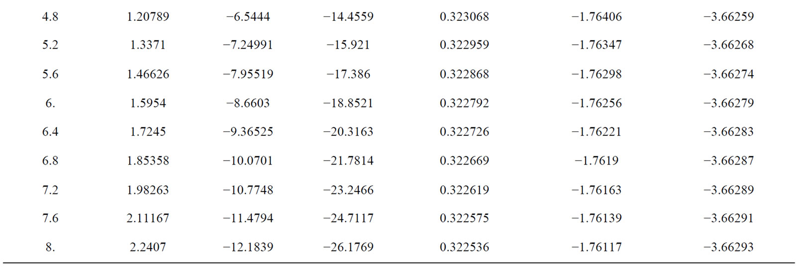
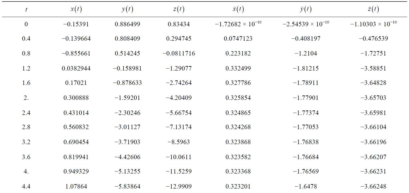
Table 2. The values of sidereal Cartesian coordinates and velocities.
3) Using the initial conditions from step 1 to solve numerically the above differential system of step 2 for
 , (note that
 ).
).
4) Using  from step 3 and the direct transformations of Equations (7) and (8) to compute numerically
  and
and 
 .
.
5) End.
4.2. Numerical Example
Consider the initial values
applying the above procedure we get the results as displayed in Tables 1 and 2.
4.3. Graphical Representations
Figure 1 illustrates the time variations of the two sidereal coordinate systems  (left) and
  (right).
5. Conclusion
In this paper of the series, the equations of motion for the spatial circular restricted three-body problem in sidereal spherical coordinates system were established. Initial value procedure that can be used to compute both the spherical and Cartesian sidereal coordinates and velocities was also developed. The application of the procedure
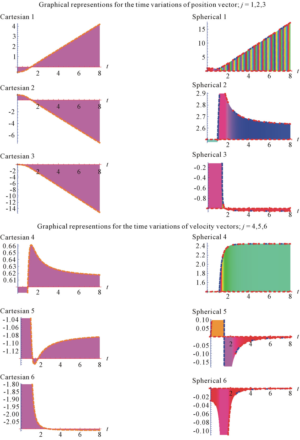
Figure 1. The time variations of the two sidereal coordinate systems (x, y, z) (left) and (u1, u2, u3) (right).
was illustrated by numerical example and graphical representations of the variations of the two sidereal coordinate systems.
REFERENCES
- M. A. Sharaf and A. A. Alshaery, “Restricted ThreeBody Problem in Cylindrical Coordinates System, (Paper I),” Journal of Applied Mathematics, 2012, in Press.
- V. Szebehely, “Theory of Orbits,” Academic Press, New York, 1967.
NOTES
*Corresponding author.