Applied Mathematics
Vol. 3 No. 5 (2012) , Article ID: 19048 , 8 pages DOI:10.4236/am.2012.35061
Variational Iterative Method Applied to Variational Problems with Moving Boundaries
Department of Applied Mathematics, Ferdowsi University of Mashhad, Mashhad, Iran
Email: fatemeghomanjani@gmail.com, s_gh333@yahoo.com
Received January 3, 2012; revised March 19, 2012; accepted March 26, 2012
Keywords: Variational Iterative Method; Variational Problems; Moving Boundaries; Isoperimetric Problems
ABSTRACT
In this paper, He’s variational iterative method has been applied to give exact solution of the Euler Lagrange equation which arises from the variational problems with moving boundaries and isoperimetric problems. In this method, general Lagrange multipliers are introduced to construct correction functional for the variational problems. The initial approximations can be freely chosen with possible unknown constant, which can be determined by imposing the boundary conditions. Illustrative examples have been presented to demonstrate the efficiency and applicability of the variational iterative method.
1. Introduction
In modeling a large class of problems arising in science, engineering and economics, it is necessary to minimize amounts of a certain functional. Because of the important role of this subject, special attention has been given to these problems. Such problems are called variational problems, see [1,2].
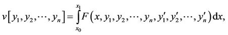
The simplest form of a variational problem can be considered as
 (1)
(1)
where  is the functional which its extremum must be found. Functional
  can be considered by two kinds of boundary conditions. In the fixed boundary problems, the admissible function
  must satisfy following boundary conditions
 (2)
(2)
In moving boundary problems, at least one of the boundary points of the admissible function is movable along a boundary curve. Further more many applications of the calculus of variations lead to problems in which not only boundary conditions, but also a quite different type of conditions known as constraints, are imposed on the admissible function. The necessary condition for the admissible solutions of such problems has to satisfy the Euler-Lagrange equation which is generally nonlinear.
In this work we consider He’s variational iterative method as a well known method for finding both analytic and approximate solutions of differential equations. Here, the problem is initially approximated with possible unknowns. Then a correction functional is constructed by a general Lagrange multiplier, which can be identified optimally via the variational theory [3].
Variational iterative method is applied on various kinds of problems [4-31].
Author of [32] solved variational problems with moving boundaries with Adomian decomposition method. Variational iterative method was applied to solve variational problems with fixed boundaries (see [11,27,30]). In this work we obtain exact solution of variational problems with moving boundaries and isoperimetric problems by variational iterative method. In fact, variational iterative method is applied to solve the Euler-Lagrange equation with prescribed boundary conditions. To present a clear overview of the procedure several illustrative examples are included.
2. Variational Iterative Method
In variational iterative method which is stated by He [3], solutions of the problems are approximated by a set of functions that may include possible constants to be determined from the boundary conditions. In this method the problem is considered as
 , (3)
, (3)
where  is a linear operator, and
  is a nonlinear operator.
  is an inhomogeneos term. By using the variational iterative method, the following correct functional is taken into account
 (4)
(4)
where  is Lagrange multiplier [5], the subscript n denotes the n-th approximation,
  is as a restricted variation i.e.
  [6-8]. Taking the variation from both sides of the correct functional with respect to yn and imposing
 , the stationary conditions are obtained. By using the stationary conditions the optimal value of the
  can be identified.
The successive approximation  can be established by determining a general lagrangian multiplier
  and initial solution
 . Since this procedure avoids the discretization of the problem, it is possible to find the closed form solution without any round off error.
In the case of m equations, the equations are rewritten in the form of:
 (5)
(5)
where  is a linear with respect to
 , and
, and  is nonlinear part of the ith equation. In this case the correct functionals are produced as
 (6)
(6)
and the optimal values of the  are obtained by taking the variation from both sides of the correct functionals and finding stationary conditions using
 。
。
3. Statement of the Problem
3.1. Moving Boundary Problems
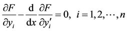
The necessary condition for the solution of problem (1) is to satisfy the Euler-Lagrange equation
 (7)
(7)
The general form of the variational problem (1) is
 (8)
(8)
Here, the necessary condition for the extermum of the functional (8) is to satisfy the following system of second-order differential equations
 (9)
(9)
In fixed boundary problems, Euler-Lagrange equation must be considered by the boundary conditions, but for the problems with variable boundaries, Euler-Lagrange equation must satisfy natural boundary conditions or transversality conditions which will be described in the following theorems.
For the problems with variable boundaries, we have two cases:
Type 1: As the first case, those problems are considered for which at least one of the boundary points move freely along a line parallel to the y-axis. Indeed at this point  is not specified. In this case all admissible functions have the same domain
  and satisfy the Euler-Lagrange equation in this interval. Furthermore such functions have to satisfy conditions called natural boundary conditions stated in the following theorem.
Theorem 3.1. Suppose the function  in
in , yields a relative minimum of the functional (1) that for which
 ,
,  is arbitrary (free right endpoint) and
 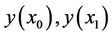 are arbitrary (free endpoints). Then
  satisfies, the following natural boundary conditions, respectively:
 (10)
(10)
or
 (11)
(11)
Type 2: For the second case, the beginning and end points (or only one of them) can move freely on given curves . In this case, a function
 is required, which emanates at some
  from the curve
  and terminates for some
  on the curve
  and minimizes the functional (1). In this problem, the points
  are not known, and they must satisfy the necessary conditions called transversality conditions, described in the following theorem.
Theorem 3.2. If the function
 , which emanates at some
 from the curve
  and terminates for some
  on the curve
  , yields a relative minimum for functional (1), where
 , R being a domain in the
  space that contains all lineal elements of
 , then it is necessary that
 to satisfy the Euler-Lagrange equation in the interval
  and at the point of exit and the point of entrance, the following transversality conditions to be satisfied:
 (12)
(12)
 (13)
(13)
In the case that one of the points is fixed, then the transversality condition has to be held at the other point.
One can consider transversality conditions for the problems with more than one unknown functions. For example, in to minimize two dimensional case, a vector function  is looked for such that
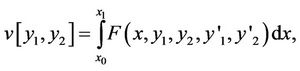 (14)
(14)
in which 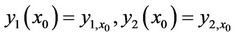 and the endpoint lies on a two-dimensional surface that is given by
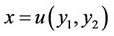 . Here the transversality conditions at
  are:
are:
 (15)
(15)
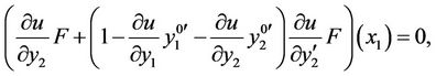 (16)
(16)
In which  is an admissible vector function.
For further information on transversality conditions, specially for the proofs of Theorems 3.1 and 3.2 and conditions (15), (16), see [2].
Example 3.1. Consider the following functional:
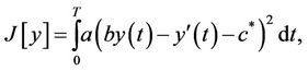 (17)
(17)
In which  and
and  is the amount of a capital at time t (see [1]).
Here, the capital stock  at the initial time
  of the planning period is assumed to be known:
 ; on the other hand, the planner won’t wish to explain how large the capital would be at time
 . Therefore, there is a variational problem with free right endpoint. Here we let
 , and
, and  which has the analytical solution
  The corresponding Euler-Lagrange equation is:
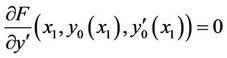
Now natural boundary condition at  is as following:
Therefore, the following boundary conditions are:
 (18)
(18)
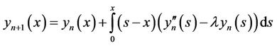
By using variational iterative method we consider the following functional is considered:
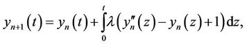
Taking the variation from both sides of the correct functional with respect to  given:
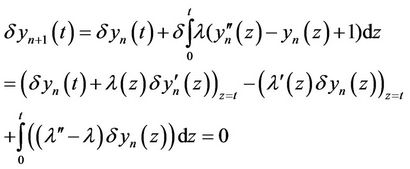
For all variations  and
and . The following stationary conditions are obtained:
 ,
,
So that . Therefore iterative formula can be found as:
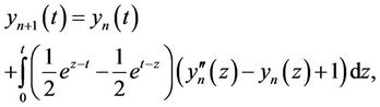
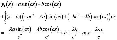
If  then
then
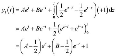
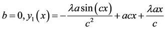
By imposing (18) 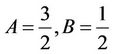 are resulted. Which yields the exact solutions of the problem (see Figure 1).
Example 3.2. We want to find the shortest distance from the point  to the sphere
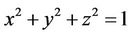
This problem is reduced to optimize the following functional:
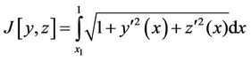 (19)
(19)
where the point  must lie on the sphere, with the exact solution
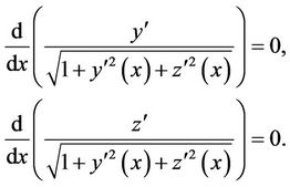
 , see [33]. The corresponding Euler Lagrange equations for this problem
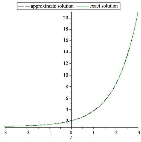
Figure 1. The graphs of approximated and exact solution for Example 3.1.
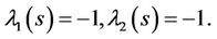
are:
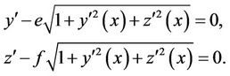
So that
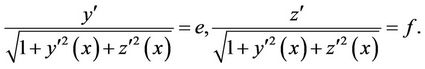
In above equations “e” and “f” are constant, so they can be rewritten as:
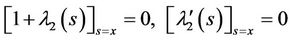
The transversality conditions are:
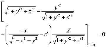 (20)
(20)
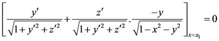 (21)
(21)
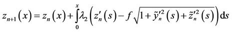
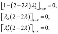
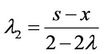
By using variational iteration method results:
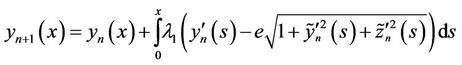
and
The variation from both sides of above equations for finding the optimal value of  is:
is:
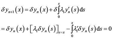
and
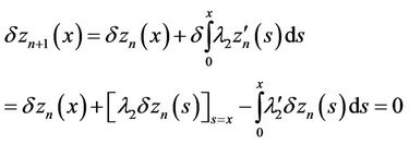
Therefore
 .
.
and
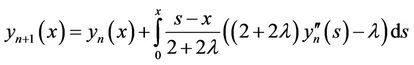
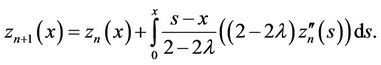
which yields:
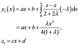
So that the following iterative formulas are obtained:
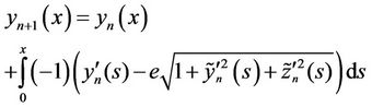
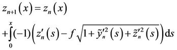
If 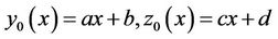 then we have:
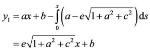
and
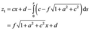
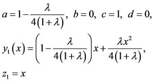
By choosing ,
,
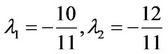
Imposing (20) and (21) lead to,  therefore:
which is the exact solution.
3.2. Isoperimetric Problems
Assume that two functions  and
and  are given. Among all curves
  along which the functional
assumes a given value l, determine the one for which the functional

Gives an extermal value. Suppose that F and G have continuous first and second partial derivatives for  and for arbitrary values of the variables
  and
and .
.
Euler’s theorem: If a curve  extremizes the functional J
  under the conditions
and if  is not an extremal of the functional K, there exists a constant
  such that the curve
  is an extremal of the functional
The necessary condition for the solution of this problem is to satisfy the Euler-Lagrange equation
with given boundary conditions in which  for further information (see [2]).
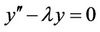
Example 3.3. It is aimed to find the minimum of the functional
 (22)
(22)
Such that
 (23)
(23)
and
 (24)
(24)
With exact solution  [19]. According to the following auxiliary functional:
and the corresponding Euler-Lagrange equation:
so
By applying He’s variational iterative method results
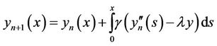
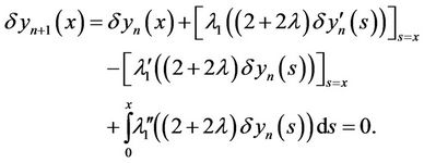
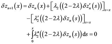
To find the optimal value of  following equation is required:
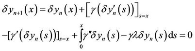
Therefore, the stationary conditions are obtained in the following form:
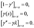
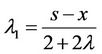
which yields

and the desired sequence is
By choosing 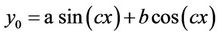
Imposing (24) on this function given
 (25)
(25)
If  then from (24)
  but from (23)
  which is a contradiction.
Now imposing (24), we have: 
so  and it is known that in this case imposing (24) on the Euler Lagrange equation yields
Hence:
and from (23) . But y must be extremal when
  , therefore:
As it is observed that this solution is equal to exact solution (see Figure 2).
Example 3.4. The objective is to find an extremum of the functional
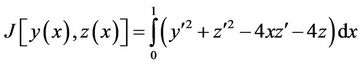 (26)
(26)
Such that
 (27)
(27)
and
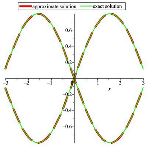
Figure 2. The graphs of approximated and exact solution for Example 3.3.
 (28)
(28)
With exact solution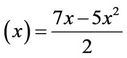 ,
,  , see [33]. By having the following auxiliary functional:
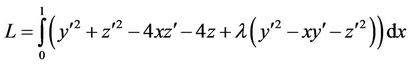
The system of Euler-Lagrange equations is in the form:
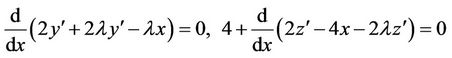 .
.
So
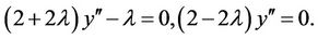
By using Homotopy variational iterative method gives:
Now
therefore

Hence
and
so
So  is obtained as:
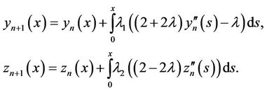
and the following iterative equations are obtained:
 ,
,
By choosing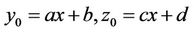 :
:
And by imposing (28) on this functions:
from (27):
And consequently:
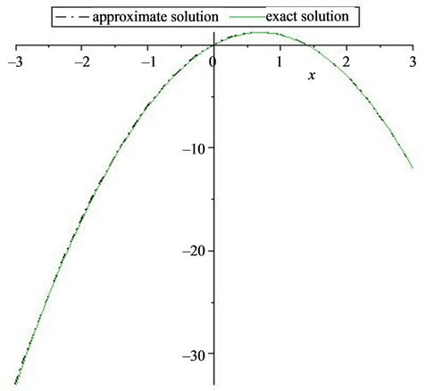
Figure 3. The graphs of approximated and exact solution for Example 3.4.
 .
.
which is the exact solution (see Figure 3).
4. Conclusion
The He’s variational iterative method is an efficient method for solving various kinds of problems. In this paper variational iterative method is employed for finding the minimum of a functional with moving boundaries and isoperimetric problems. Using He’s variational iterative method the solution of the problem is provided in a closed form. Since this method does not need to the discretize of the variables, there is no computational round off error. Moreover, only a few numbers of iterations are needed to obtain a satisfactory result.
REFERENCES
- P. G. Engstrom and U. Brechtken-Manderschied, “Introduction to the Calculus of Variations,” Chapman and Hall/CRC, New York, 1991.
- A. Saadatmandi and M. Dehghan, “He’s Variational Iteration Method for Solving a Partial Differential Equation Arising in Modeling of Water Waves,” Zeitschrift für Naturforschung, Vol. 64, 2009, pp. 783-787.
- J. H. He, “Variational Iteration Method a Kind of NonLinear Analytical Technique: Some Examples,” International Journal of Nonlinear Mechanics, Vol. 34, No. 4, 1999, pp. 699-708. doi:10.1016/S0020-7462(98)00048-1
- M. A. Abdou and A. A. Soliman, “Varitional Iteration Method for Solving Burgers’ and Coupled Burgers’ Equations,” Journal of Computational and Applied Mathmatics, Vol. 181, 2005, pp. 45-251.
- J. Biazar and H. Ghazvini, “He’s Variational Iteration Method for Solving Hyperbolic Differential Equations,” International Journal of Nonlinear Sciences and Numerical Simulation, Vol. 8, 2007, pp. 311-314.
- M. Dehghan and M. Tatari, “The Use of He’s Variational Iteration Method for Solving a Fokker Planck Equation,” Physica Scripta, Vol. 74, No. 3, 2006, pp. 310-316. doi:10.1088/0031-8949/74/3/003
- M. Dehghan and A. Saadatmandi, “Variational Iteration Method for Solving the Wave Equation Subject to an Integral Conservation Condition,” Chaos, Solitons and Fractals, Vol. 41, No. 3, 2009, pp. 448-1453. doi:10.1016/j.chaos.2008.06.009
- M. Dehghan and F. Shakeri, “Approximate Solution of a Differential Equation Arising in Astrophysics Using the Variational Iteration Method,” New Astronomy, Vol. 13, No. 1, 2008, pp. 53-59. doi:10.1016/j.newast.2007.06.012
- M. Dehghan and F. Shakeri, “Application of He’s Variational Iteration Method for Solving the Cauchy Reaction-Diffusion Problem,” Journal of Computational and Applied Mathematics, Vol. 214, No. 2, 2008, pp. 435-446. doi:10.1016/j.cam.2007.03.006
- M. Dehghan and R. Salehi, “The Use of Variational Iteration Method and Adomian Decomposition Method to Solve the Eikonal Equation and Its Application in the Reconstruction Problem,” Communications in Numerical Methods in Engineering, in press.
- M. Dehghan and M. Tatari, “The Use of Adomian Decomposition Method for Solving Problems in Calculus of Variations,” Mathematical Problems in Engineering, Vol. 2006, 2006, pp. 1-12. doi:10.1155/MPE/2006/65379
- M. Dehghan and M. Tatari, “Identifying an Unknown Function in a Parabolic Equation with over Specified Data via He’s Variational Iteration Method,” Chaos, Solitons and Fractals, Vol. 36, 2008, pp. 57-166.
- J. H. He, “Variational Iteration Method for Autonomous Ordinary Differential Systems,” Applied Mathematics and Computation, Vol. 114, No. 2-3, 2000, pp. 115-123. doi:10.1016/S0096-3003(99)00104-6
- J. H. He and X. H. Wu, “Variational Iteration Method: New Development and Applications,” Computers and Mathematics with Applications, Vol. 54, No. 7-8, 2007, pp. 881-894. doi:10.1016/j.camwa.2006.12.083
- J. H. He, “Variational Iteration Method: Some Recent Results and New Interpretations,” Journal of Computational and Applied Mathematics, Vol. 207, No. 1, 2007, pp. 3-17. doi:10.1016/j.cam.2006.07.009
- J. H. He, Variational Iteration Method for Delay Differential Equations,” Communications in Nonlinear Science and Numerical Simulation, Vol. 2, No. 4, 1997, pp. 235- 236. doi:10.1016/S1007-5704(97)90008-3
- J. H. He, “Approximate Solution of Nonlinear Differential Equations with Convolution Product Nonlinearities,” Computer Methods in Applied Mechanics and Engineering, Vol. 167, No. 1-2, 1998, pp. 69-73. doi:10.1016/S0045-7825(98)00109-1
- J. H. He, “Approximate Analytical Solution for Seepage Flow with Fractional Derivatives in Porous Media,” Computer Methods in Applied Mechanics and Engineering, Vol. 167, No. 1-2, 1998, pp. 57-68. doi:10.1016/S0045-7825(98)00108-X
- M. Inc, “Numerical Simulation of KdV and mKdV Equations with Initial Conditions by the variational Iteration Method,” Chaos, Solitons and Fractals, Vol. 34, No. 4, 2007, pp. 1075-1081. doi:10.1016/j.chaos.2006.04.069
- S. Momani and S. Abuasad, “Application of He’s Variational Iteration Method to Helmholtz Equation,” Chaos, Solitons and Fractals, Vol. 27, No. 5, 2006, pp. 1119- 1123. doi:10.1016/j.chaos.2005.04.113
- S. Momani and Z. Odibat, “Analytical Approach to Linear Fractional Partial Differential Equations Arising in Fluid Mechanics,” Physics Letters A, Vol. 355, No. 4-5, 2006, pp. 271-279. doi:10.1016/j.physleta.2006.02.048
- H. Ozer, “Application of the Variational Iteration Method to the Boundary Value Problems with Jump Discontinuities Arising in Solid Mechanics,” International Journal of Nonlinear Sciences and Numerical Simulation, Vol. 8, 2007, pp. 513-518.
- Z. M. Odibat and S. Momani, “Application of Variational Iteration Method to Nonlinear Differential Equations of Fractional Order,” International Journal of Nonlinear Sciences and Numerical Simulation, Vol. 7, 2007, pp. 27- 34. doi:10.1515/IJNSNS.2006.7.1.27
- H. Sagan, “Introduction to the Calculus of Variations,” Courier Dover Publications, 1992.
- F. Shakeri and M. Dehghan, “Numerical Solution of the Klein-Gordon Equation via He’s Variational Iteration Method,” Nonlinear Dynamics, Vol. 51, No. 1-2, 2008, pp. 89-97. doi:10.1007/s11071-006-9194-x
- F. Shakeri and M. Dehghan, “Solution of a Model Describing Biological Species Living Together Using the Variational Iteration Method,” Mathematical and Computer Modeling, Vol. 48, No. 5-6, 2008, pp. 685-699. doi:10.1016/j.mcm.2007.11.012
- M. Tatari and M. Dehghan, “Solution of Problems in Calculus of Variations via He’s Variational Iteration Method,” Physics Letters A, Vol. 362, No. 5-6, 2007, pp. 401-406. doi:10.1016/j.physleta.2006.09.101
- M. Tatari and M. Dehghan, “Improvement of He’s Variational Iteration Method for Solving Systems of Differential Equations,” Computers and Mathematics with Applications, Vol. 58, No. 11-12, 2009, pp. 2160-2166. doi:10.1016/j.camwa.2009.03.081
- M. Tatari and M. Dehghan, “On the Convergence of He's Variational Iteration Method,” Journal of Computational and Applied Mathematics, Vol. 207, No. 1, 2007, pp. 121- 128. doi:10.1016/j.cam.2006.07.017
- S. A. Youse and M. Dehghan, “The Use of He’s Variational Iteration Method for Solving Variational Problems,” International Journal of Computer Mathematics, Vol. 87, No. 6, 2010. doi:10.1080/00207160802283047
- A. M. Wazwaz, “A Comparison between the Variational Iteration Method and Adomian Decomposition Method,” Journal of Computational and Applied Mathematics, Vol. 207, No. 1, 2007, pp. 129-136. doi:10.1016/j.cam.2006.07.018c
- R. Memarbashi, “Variational Problems with Moving Boundaries Using Decomposition Method,” Mathematical Problems in Engineering, Vol. 2007, 2007, Article ID 10120.
- M. L. Krasnov, G. I. Makarenko and A. I. Kiselev, “Problems and Exercises in the Calculus of Variations,” Mir Publisher, Moscow, 1964.