Applied Mathematics
Vol. 3 No. 2 (2012) , Article ID: 17379 , 8 pages DOI:10.4236/am.2012.32018
Invariant Relative Orbits Taking into Account Third-Body Perturbation
1Department of Astronomy, Faculty of Science, Cairo University, Cairo, Egypt
2Observatoire de la Côte d’Azur, Grasse, France
Email: walid_rahoma@yahoo.com
Received October 12, 2011; revised December 19, 2011; accepted December 27, 2011
Keywords: Invariant Relative Orbits; Third-Body Perturbation; Hamiltonian
ABSTRACT
For a satellite in an orbit of more than 1600 km in altitude, the effects of Sun and Moon on the orbit can’t be negligible. Working with mean orbital elements, the secular drift of the longitude of the ascending node and the sum of the argument of perigee and mean anomaly are set equal between two neighboring orbits to negate the separation over time due to the potential of the Earth and the third body effect. The expressions for the second order conditions that guarantee that the drift rates of two neighboring orbits are equal on the average are derived. To this end, the Hamiltonian was developed. The expressions for the non-vanishing time rate of change of canonical elements are obtained.
1. Introduction
Formation flying is a key technology enabling a number of missions which a single satellite cannot accomplish: from remote sensing to astronomy. The relative motion, which shows no drift even in presence of a large disturbance, could be a very attractive solution. To maintain the formation and constellation, the relative drifts due to the perturbation between the spacecraft should be carefully considered. Invariant Relative Orbits shows no drift between the spacecraft due to the perturbation even if in presence of a large disturbance.
The literature is wealth with works dealing with designing certain invariant relative orbits for spacecraft flying formations, and it seems worth to sketch some of the most relevant works. Schaub and Alfriend [1] presented a method to establish J2 invariant relative orbits for spacecraft formation flying applications. They designed relative orbit geometry using differences in mean orbit elements. Two constraints on the three momenta element differences are derived. Zhang and Dai [2] removed the drifts by adjusting the semi-axis of the follower satellite and obtained a similar conclusion. By means of Routh transformation and dynamical system theory, Koon and Marsden [3] developed a method to find the  invariant orbit. Then Li and Li [4] and Meng et al. [5] concluded, from the point of view of relative orbital elements, that the drifts of relative orbit result from the orbital inclination and right ascension of ascending node of the two satellites. Biggs and Becerra [6] proposed a method to determinate the J2 invariant orbit with the leader’s orbit of zero inclination based on the targeting method in chaos dynamics. Abd El-Salam et al. [7] used the Hamiltonian framework to construct an analytical method to design invariant relative constellation orbits due to the zonal harmonics
 ;
; ;
;  up to the second order, assuming
  being of order 1.
Our propose was to extend Schaub and Alfriend [1] and Abd El-Salam et al. [7] model by adding the effect of the third body which have important at high altitude. Using the Hamiltonian framework, the perturbations can be easily added. The Hamiltonian of the problem was constructed by considering the effect of the third body of . The expressions for the time rate of change of the secular elements are obtained, second order conditions are established between the differences in momenta elements (semi-major axis, eccentricity and inclination angle) that guarantee that the drift rates of two neighboring orbits are equal on the average.
2. Hamiltonian Approach
There are several ways to derive the equations of motion for any such system. We emphasized on the Hamiltonian structure for this system. The Hamiltonian formulation allows for additional conservative forces to be added to the Hamiltonian, thus the addition of complexity to the model can be incorporated with ease. Non-conservative forces can be added in the momenta equations of motion. The Hamiltonian equations of motion allows us to directly use control and simulation techniques.
Notations in the whole text, we use the well-known keplerian elements: the semi-major axis a, the eccentricity e, the inclination , the right ascension of ascending node
 , the argument of perigee
 , and the mean anomaly M. We also use the true anomaly f and an intermediary variable
 .
.
The Hamiltonian in the present framework can be written in the form
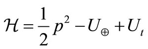 (1)
(1)
where  is the force function due to the Earth’s gravitational potential, and p is the canonical momentum vector and
  the disturbing function due to the effect of perturbing body.
2.1. Influence of Oblateness Perturbations
The actual shape of the Earth is that of an eggplant. The center of mass does not lie on the spin axis and neither the meridian nor the latitudinal contours are circles. The net result of this irregular shape is to produce a variation in the gravitational acceleration to that predicted using a point mass distribution. The Earth’s gravitational potential is usually expressed by the following expression (Vinti’s potential)
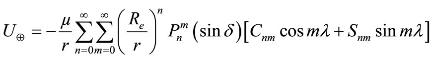
where  is the equatorial radius of the Earth,
 is the Earth’s gravitational parameter where
  is the gravitational constant;
 are the geocentric coordinates of the satellite with
  measured east of Greenwich;
 and
and  are harmonic coefficients;
 are associated Legendre Polynomials.
In the potential function, the terms with ,
,  and
and  correspond respectively to zonal, tesseral and sectorial harmonics. The Earth gravitational potential can be rewritten, up to second order in
 , truncating the series at
 , as, Abd El-Salam et al. [7]
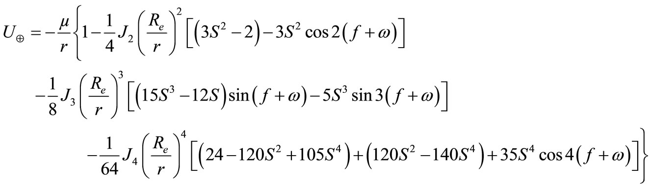 (2)
(2)
where  and
and  is the zonal harmonic coefficients.
2.2. Third Body Perturbation
The effect of the third body in the motion of an artificial satellite have became particularly interesting now, when space debris imposes a serious threat to space activities. These perturbations are the most important mechanism of delivering major Earth orbiting objects into the regions where the atmosphere can start their decay.
If it is assumed that the main body; Earth; with mass  is fixed in the center of the reference system x-y. The perturbing body, with mass
  is in an elliptic orbit with semi-major axis,
  , eccentricity
 , and mean motion
 , given by the expression
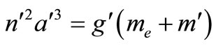 ,
,  and
and  are the radius vectors of the satellite and
  (assuming
 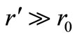 ), and
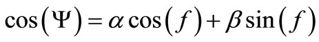
  is the angle between these radius vectors. The disturbing function (using the tradition expansion in Legendre polynomials) due to the third body is given by, Domingos et al. [8],
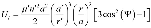 (3)
(3)
where 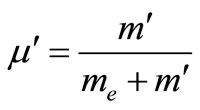 and
and
with


Using the Delaunay canonical-variables  defined by
 Mean anomaly
 Argument of the Perigee
 Longitude of ascending node
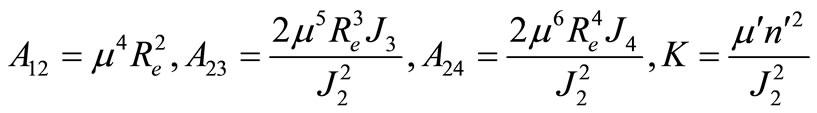
Considering  as a small parameter of the problem, the orders of magnitude, up to the second order, of the involved parameters are defined as follows:
 , and let us define the dimensionless parameters as
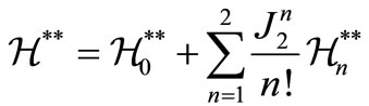
The Hamiltonian, Equation (1) up to the second order, can now be expressed as a power series in  as follows
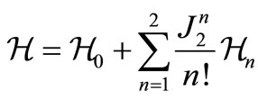 (4)
(4)
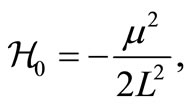
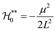
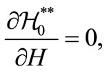
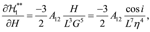
where  represents the unperturbed part of the problem,
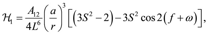
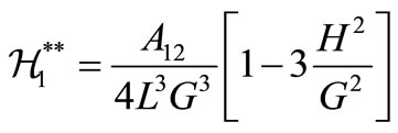
  is the perturbation:
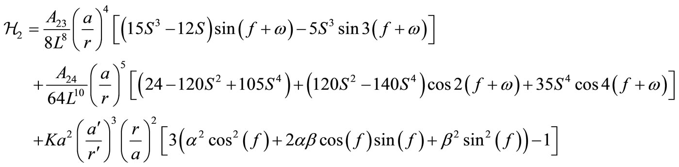
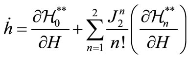
Now we need to eliminate the short as well as the long periodic terms of the satellite motion in addition to the short periodic terms of the distance perturbing body. Using the perturbation technique based on Lie series and Lie transform, Kamel [9], the transformed Hamiltonianfor different orders 0, 1, 2 can be written as, Abd ElSalam et al. [7] and Domingos et al. [8].
 (5)
(5)
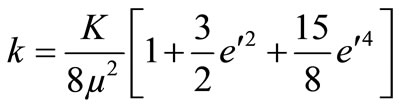
with
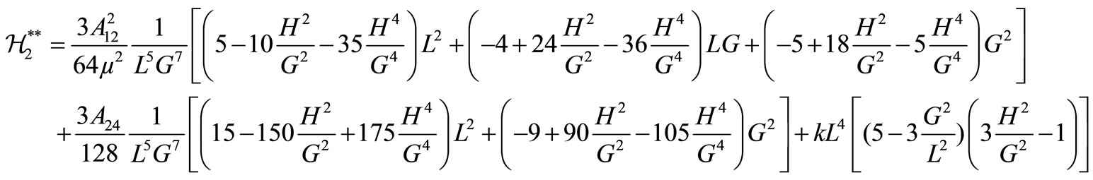
where
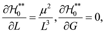
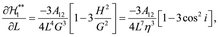
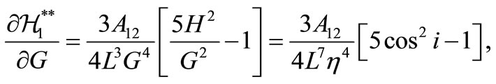
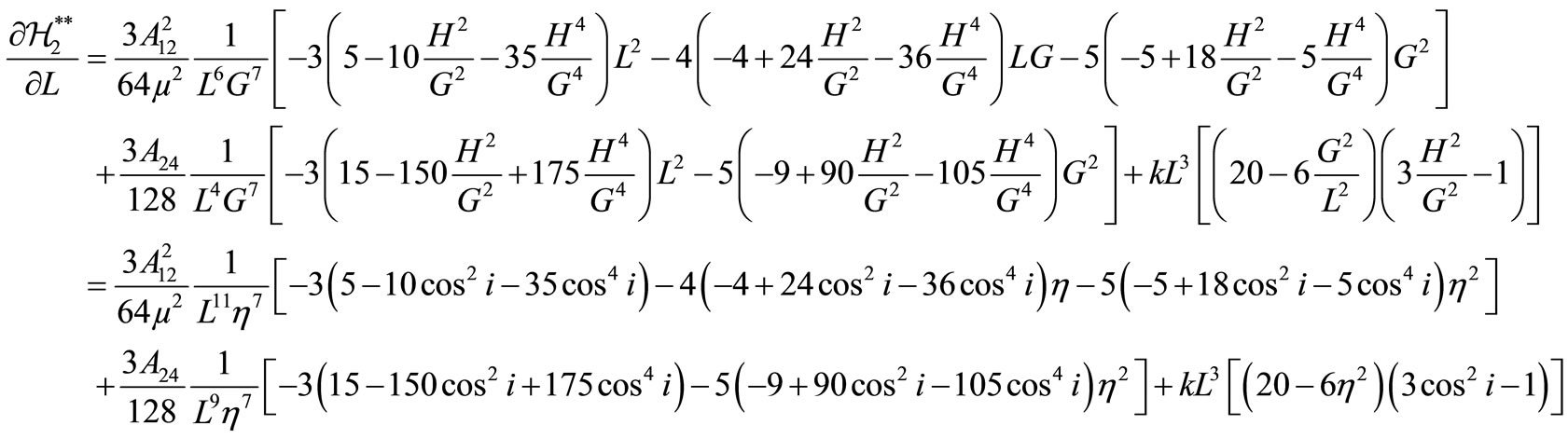
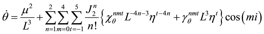
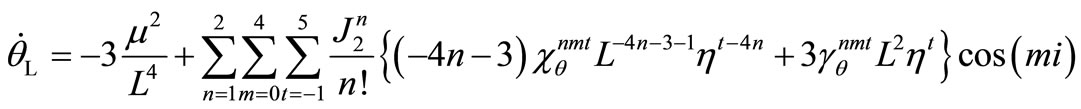
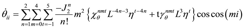
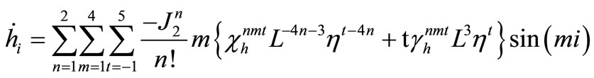
Using the Hamiltonian canonical equations of the motion, to write , argument of mean latitude (
 ) is the sum of the mean anomaly and the argument of perigee (i.e.
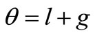 ), as
), as
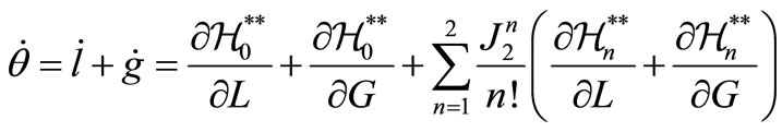 (6)
(6)
with
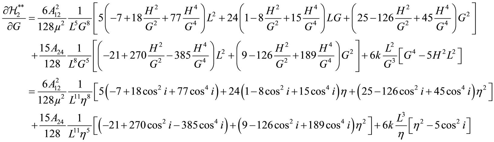
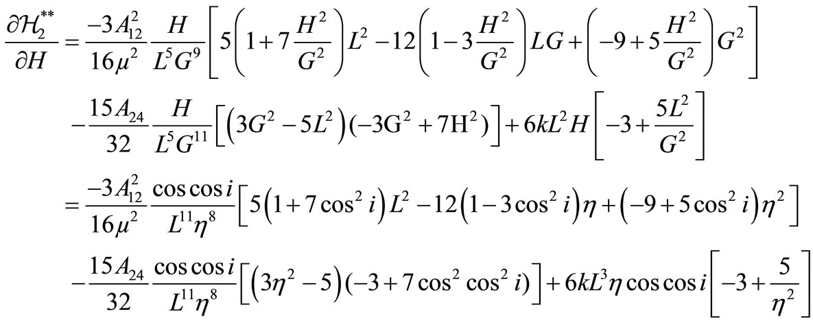
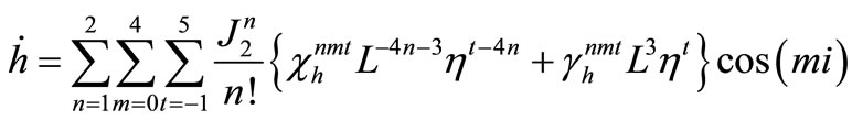
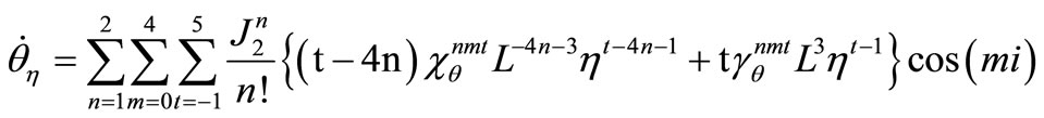
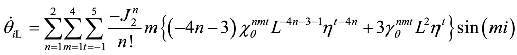
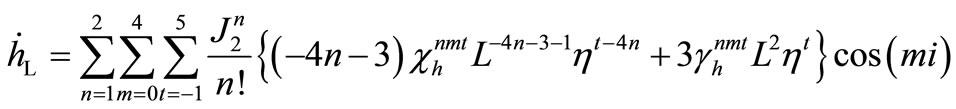
and the secular drift rates of the longitude of the ascending node, :
:
 (7)
(7)
with
3. Constraints for Invariant Orbits
In order to prevent two neighboring orbits from drifting apart, the average secular growth needs to be equal. Short period oscillations can be ignored here since these are only “temporary” deviations. The long period rates appear secular over a few weeks and they are .
.
Since the mean angle quantities  and
and  do not directly contribute to the secular growth, their values can be chosen at will. However, the mean momenta values
  and H (and therefore implicitly
  and
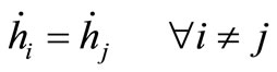
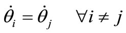
and ) must be carefully chosen to match the secular drift rates. To keep the satellites from drifting apart over time, it would be desirable to match all three rates
 . We impose the condition that the relative average drift rate of the angle between the radius vectors be zero. This results in
 (9)
(9)
 (10)
(10)
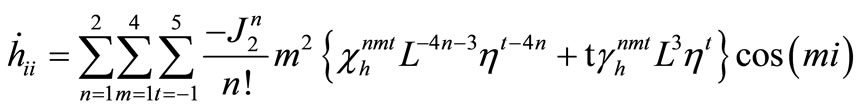
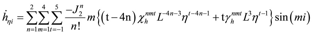
Now  and
and  can be rewritten as
 (11)
(11)
 (12)
(12)
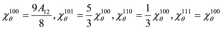
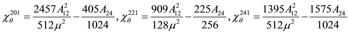
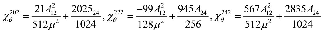
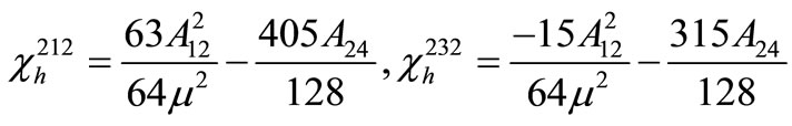
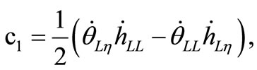
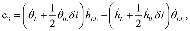
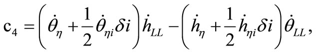
where the non-vanishing coefficients  and
and  are computed in Appendix I.
Let the reference mean orbit elements be denoted with the subscript “0”. The drift rate  of a neighboring orbit can be written as a series expansion about the reference orbit element, here it is enough to keep the second order only, as
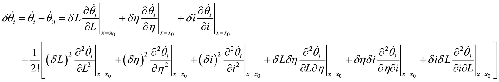 (13)
(13)
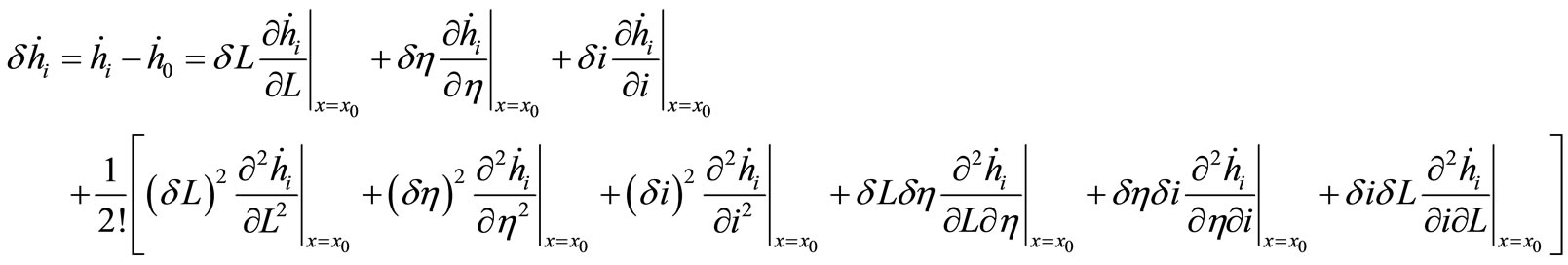 (14)
(14)
where we make use of the fact that  and
and  only, also supposing that
  is the difference in mean latitude rates,
 and
and 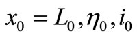
Note that this theory will lead to an analytical second order conditions on the mean orbit elements. To establish a more precise set of orbit elements satisfying Equations
(9) and (10), either  or
or  could be chosen and the remaining two momenta orbit element differences found through a numerical root solving technique. However, the analytical second order conditions provide reasonably accurate solutions to these two constraints equations and provide a wealth of insight into the behavior of Earth potential and third body effect invariant relative orbits.
The required derivatives can be evaluated as


and


where  and
and  with
with .
.
To enforce equal drift rates and
and  between neighboring orbits, we must set
  and
and  equal to zero in expanded Equations (13) and (14), yields
 (15)
(15)
 (16)
(16)
Equations (15) and (16) are two simultaneous nonlinear algebraic equations in three unknowns, namely . When one of these three unknowns is assumed known (say
 ), these two equations can be solved as:
Multiplying Equation (15) by  and Equation (16) by
  and then subtracting yields
 (17)
(17)
where

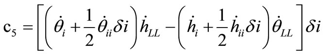 .
.
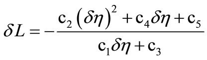
Substituting Equation (17) into Equation (15) yields an algebraic equation of fourth degree in  only in the form
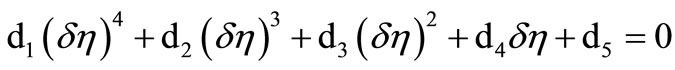 (18)
(18)
where
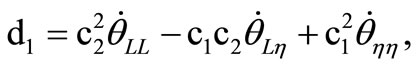
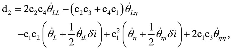
 .
.
4. Solution of the Quartic Equation (18)
The roots of the quartic Equation (18) can be written as
where
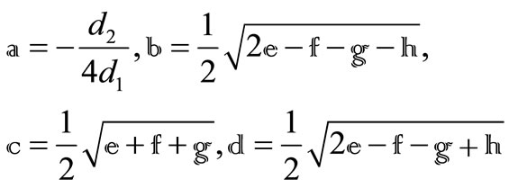
with
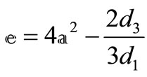 ,
, 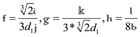
where
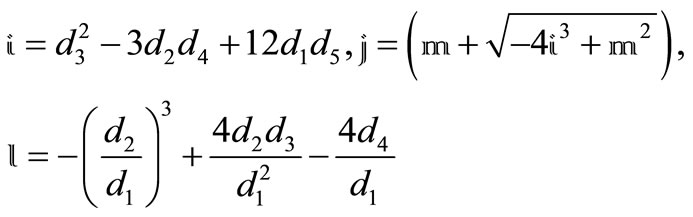
and
 .
.
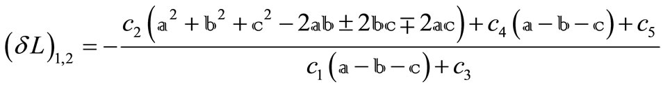
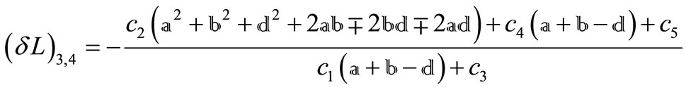
Substituting the four roots ’s into Equation (17) yields the four constraints
 ’s that guarantee the invariance of the relative motion of certain satellite constellation
5. Conclusion
Accurate modeling of relative motion dynamics for initial conditions close to the leader satellite is essential for flying formation. Therefore, the solutions of interest are restricted to a specific set of initial conditions that lead to periodic motion, such that the satellites do not drift apart. This paper showed an analytical expression to secular drift rates due to oblate Earth model, truncating its potential series at , and third body effect and set it equal between two neighboring orbits. It followed the same steps used before in Abd El-Salam et al. [7] for the Earth model so the calculation of Abd El-Salam et al. [7] and Schaub and Alfriend [1] is a special case from this calculations. The variation in the inclination (
 ) can be chosen at will for the nominal inclination, and the variations in both the eccentricity (
 ) and semi-major axis (
 ) from their nominal values are set to zero. Noted that these constraint conditions are not justified near the critical inclination angle. Using
  instead of
  to avoid the singularity when
  but for
  the nonsingular elements must be used. Future developments of this approach to the formation flying problem include another perturbation forces like solar radiation and lunisolar effects.
6. Acknowledgements
The first author wish to express his appreciation for the support provided by the French government under the No de dossier: 688028B, No affiliation: 194264/733177.
The authors gratefully thank referees for their helpful, suggestions and comments.
REFERENCES
- H. Schaub and K. Alfriend, “J2 Invariant Relative Orbits for Spacecraft Formations,” Celestial Mechanics and Dynamical Astronomy, Vol. 79, No. 2, 2001, pp. 77-95. doi:10.1023/A:1011161811472
- Y. Zhang and J. Dai, “Satellite Formation Flying with J2 Perturbation,” Journal of National University of Defense Technology, Vol. 24, No. 2, 2002, pp. 6-10.
- W. S. Koon and J. E. Marsden, “J2 Dynamics and Formation Flight,” Proceedings of AIAA Guidance, Navigation, and Control Conference, Montreal, August 2001, p. 4090.
- X. Li and J. Li, “Study on Relative Orbital Configuration in Satellite Formation Flying,” Acta Mechanica Sinica, Vol. 21, No. 1, 2005, pp. 87-94. doi:10.1007/s10409-004-0009-3
- X. Meng, J. Li and Y. Gao, “J2 Perturbation Analysis of Relative Orbits in Satellite Formation Flying,” Acta Mechanica Sinica, Vol. 38, No. 1, 2006, pp. 89-96.
- J. D. Biggs and V. M. Becerra, “A Search for Invariant Relative Satellite Motion,” 4th Workshop on Satellite Constellations and Formation Flying, Sao Jose dos Campos, 2005, pp. 203-213.
- F. A. Abd El-Salam, I. A. El-Tohamy, M. K. Ahmed, W. A. Rahoma and M. A. Rassem, “Invariant Relative Orbits for Satellite Constellations: A Second Order Theory,” Applied Mathematics and Computation, Vol. 181, No. 1, 2006, pp. 6-20. doi:10.1016/j.amc.2006.01.004
- R. C. Domingos, R. V. deMoraes and A. F. Prado, “Third-Body Perturbation in the Case of Elliptic Orbits for the Disturbing Body,” Mathematical Problems in Engineering, Vol. 2008, 2008, p. 14. doi:10.1155/2008/763654
- A. A. Kamel, “Expansion Formulae in Canonical Transformations Depending on a Small Parameter,” Celestial Mechanics and Dynamical Astronomy, Vol. 1, No. 2, 1969, pp. 190-199. doi:10.1007/BF01228838
Appendix I