Modern Economy
Vol. 3 No. 8 (2012) , Article ID: 26138 , 8 pages DOI:10.4236/me.2012.38113
Mystery of Modern Phillips Curve
Department of Economics, Rutgers University, Camden, USA
Email: jinpeng@crab.rutgers.edu
Received September 13, 2012; revised November 23, 2012; accepted December 4, 2012
Keywords: Phillips Curve; Business Cycles; Inflation; Unemployment
ABSTRACT
The modern Phillips curve is about the relationship between inflation and unemployment and has been the center of a fierce debate in economics over fifty years. This paper reports empirical evidence that uncovers some of its mysteries. The rate of inflation and the unemployment rate are closely related to business cycles. What is of interest is that no two business cycles are exactly alike; however, all business cycles are essentially alike [1,2]. Each expansion is ended by a recession induced by adverse shocks. The US economy suffers from adverse shocks all the time, but not every shock gives rise to a recession. Why do adverse shocks often induce a recession after an expansion that has lasted for a substantial duration? That is, why are double-dip recessions so rare? Here do we find important evidence in the Phillips curve that may help answer this question. We also discuss some issues related to the monetary policy and raise a few open questions about the relationship between unemployment and business cycles.
1. Introduction
A. W. Phillips [3] made the following hypothesis about the labor market:
“When the demand for a commodity or service is high relatively to the supply of it we expect the price to rise, the rate of rise being greater the greater the excess demand. Conversely when the demand is low relatively to the supply we expect the price to fall, the rate of fall being greater the greater the deficiency of demand. It seems plausible that this principle should operate as one of the factors determining the rate of change of money wage rates, which are the price of labour services. When the demand for labour is high and there are very few unemployed we should expect employers to bid wage rates up quite rapidly, each firm and each industry being continually tempted to offer a little above the prevailing rates to attract the most suitable labour from other firms and industries. On the other hand it appears that workers are reluctant to offer their services at less than the prevailing rates when the demand for labour is low and unemployment is high so that wage rates fall only very slowly. The relation between unemployment and the rate of change of wage rates is therefore likely to be highly non-linear.”
According to the Phillips hypothesis, wage rates accelerate for an increasingly tight labor market; on the other hand, they fall “only very slowly” for an increasingly slack labor market. He showed that there was an inverse relationship between the average growth rate of money wage and the average rate of unemployment, using annual data in the United Kingdom from 1861 to 1913, and demonstrated that his scatter-plot curve fitted equally well the data from 1914 to 1957, with few noted exceptions. This curve marks the birth of the Phillips curve and has a flat tail along the unemployment rate axis, an important property that is consistent with the Phillips hypothesis about wage rates for an increasingly slack labor market.
The modern Phillips curve is about the tradeoff between the rate of inflation and the rate of unemployment and has been the center of a fierce debate in economics over fifty years. The debate question is whether such a tradeoff exists. Several theories have been invented out of this debate, yet economists have not reached a uniform answer. Instead, they are in “a great divide” [4]. The Phillips curve remains a great mystery.
Economists should answer the question, not only for its own right but also for many other related questions. For example, an answer to the question may be important in order to understand how commodity and factor markets actually function during economic booms and busts. Why are there business cycles? How should the monetary and fiscal policy be conducted during an economic recession or expansion?
The Phillips curve was initially well-accepted by the Keynesians [5]; it provided a useful tool for them to determine nominal wages and unemployment. However, it was soon under an attack by the neoclassical economists and the monetarists. Milton Friedman [6] and Edmund Phelps [7,8] independently proposed a new expectations augmented Phillips curve, together with the invention of the NAIRU (non-accelerating inflation rate of unemployment) u*. The new Phillips curve focuses on the role of expectations on inflation. Inflation p(t) at time t is given by
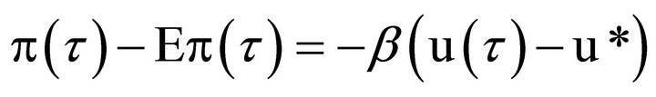
where Eπ(τ) is the expected inflation, u(t) is the rate of unemployment, and β a positive coefficient that is timeinvariant. This equation means that change in expectations shifts the Phillips curve. Under rational expectations [2], the rate of unemployment equals u*.
As a result, there is no long run tradeoff. A short run tradeoff exists only if there are misperceptions under which differentials exist between inflation p and its expectations Ep. For given expectations, inflation accelerates (decelerates) for the rate of unemployment that is below (above) the NAIRU u*. The acceleration (deceleration) in inflation is an ascending (descending) spiral between inflation and its expectations.
Persistently low rates of inflation and unemployment in the US economy during the 1980s and 1990s provided a challenge to the neoclassical school for having a unique and time-invariant u*. The new Keynesian Phillips curve (NKPC) was proposed to meet the challenge. The new Keynesians in general accept the neoclassical view that inflation expectations play a critical role on inflation; however, they insist that monopolistic competition and price rigidities are the main reason that the tradeoff exists [1,9,10].
There are many forms of NKPC. The following hybrid form [9,10] is common:

Thus, this equation means that current inflation p(t) is affected by the lagged inflation p(t − 1), the expected future inflation E(t)p(t + 1), and a measure of aggregate marginal cost mc(t). Once again, change in expectations shifts the Phillips curve. With rational expectations, inflation becomes a weighted average of marginal costs in the past and the future. Random variable e is the exogenous shock on markup. The time-invariant coefficients g, d, and l are functions of structural parameters (i.e., the percentage of monopolistic firms that keep prices rigid for certain periods and the discount factor for future utility of consumption) in an economy [9-11]. Since the aggregate marginal cost mc(t) is private information, the NKPC models use labor’s share or an output gap to replace it in estimates. Many empirical works exist in the literature. The estimates of l vary widely and are very sensitive to the sample data and the estimation methods used. Some strongly support the curve while others strongly deny it [10].
The NKPC is derived from modern dynamic stochastic general equilibrium (DSGE) models, with additional price setting equations [9-11]. A critical assumption of these models is that the US economy is on a balanced growth path with a steady economic structure, a tradition similar to the literature of real business cycles (RBS) [1]. This means that the trend growth in GDP of the US economy all follows the same economic structure. Otherwise, the models and their estimates will suffer from the Lucas Critique [12].
Our focus is on how a recession changes the Phillips curve. A recession can change both commodity and factor markets. Each recession destroys jobs for millions of people and forces a great number of firms to reorganize or reallocate resources. Some firms may exit their markets in a recession while others may seek opportunities to enter or expand.
A recession causes sector changes. A sector that grew strongly prior to a recession may not continue to grow at the same pace afterwards. There were significant changes in the growth of the high-tech sector after the 2001 recession and of the housing and mortgage markets after the 2008 recession. The economic growth after the 1991 recession was not the same as that after the 2001 recession. It is very likely that the economic growth after the 2008 and 2001 recessions won’t be the same.
A metaphor may be useful to describe the situation. When a teen grows, his deltoid and biceps muscles must grow in proportion. When a tree grows, all living branches grow together but not necessarily in proportion. Some branches may grow faster than others this year, and the luck may turn to others next year. Some branches may not survive a tough winter time while new branches pop up the next spring. The US economy grows in a trend more like a tree than like a teen. This idea of a tree growth model is in fact consistent with the Lucas Critique [12], in which Professor Robert Lucas discussed the deviations of the “true” economic structure caused by a policy change. This paper searches for evidence of possible deviations in the Phillips curve induced by a recession.
If our theory is right, we should be able to see the impact of a recession on the Phillips curve from the empirical data. To test the theory, we draw the Phillips curve for each expansion after a recession for the US economy from 1961 to 2009, covering six recessions and expansions. Our main finding is that the Phillips curve shifted and changed its pattern after each recession (Figures 2-7). No two expansions had exactly the same Phillips curve. However, the six Phillips curves we obtained did share some common features (Figures 5-7). Inflation accelerated sharply near the end of each of the six expansions. Inflation increased from its trough near the end of an expansion to its peak by 68 percent on average (Table 1). Inflation decelerated sharply when a recession hit the economy. The nearest trough in inflation after a recession was just 25 percent of the inflation rate at the peak on average (Table 2). Moreover, inflation and unemployment were observed to be positively related in the beginning of each of the six expansions. Such a positive relationship was also observed for substantial periods of time in the middle of each of the three expansions after the 1980-1982 recession.
As a result, we find that the Phillips curve holds very well near the end of each of the six expansions. However, the tradeoff fails to exist in the beginning of each of the six expansions. The tradeoff may or may not exist in the middle of an expansion.
An important use of the Phillips curve is for the monetary policy. Our finding shows that the Phillips curve is indeed important for the monetary policy at a time when it matters the most. We also find some interesting facts about business cycles. Recessions all occurred at some point as the inflation acceleration proceeded, and recoveries all occurred at some point as the
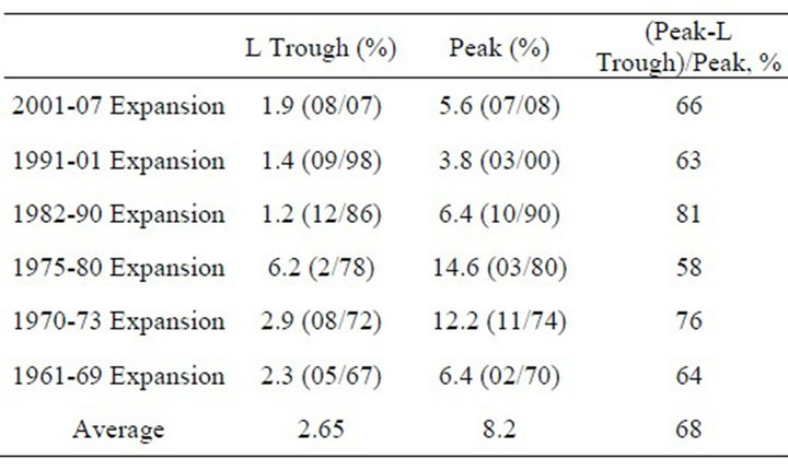
Table 1. Inflation acceleration near the end of an expansion. Peaks and troughs in inflation are read from the graph of CPI (see Figure 8). A trough in inflation is the point that is near the end of an expansion where inflation starts to climb up. In the brackets are the month and the year that inflation reaches its left trough and the peak.
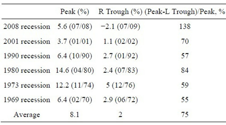
Table 2. Inflation deceleration after a recession. Peaks and troughs in inflation are read from the graph of CPI (see Figure 8). A right trough in inflation is the point that has the first lowest inflation rate after a recession. In the brackets are the month and the year that inflation reaches its peak and trough.
inflation deceleration proceeded. That is, no recession had occurred without acceleration in inflation, and no recovery had occurred without deceleration in inflation. This suggests that recessions and recoveries are closely related to acceleration and deceleration in inflation, respectively. A recession may be the consequence of a joint effort between the acceleration in inflation and adverse shocks. This may explain why business cycles are recurrent, not periodic, for expansions often have uneven lengths. It may also explain why adverse shocks often induce a recession only after an expansion has lasted for a substantial duration. We will discuss what may be the implication of our observations for conducting the monetary policy and raise a few questions about the unemployment and business cycles.
2. Data and Methodology
Our empirical work uses annual and monthly data of the US economy from 1961 to 2009. All data are from the Bureau of Labor Statistics (BLS). The inflation data are the annual and monthly CPI data with 12 month percentage change for all items and all urban consumers with base period 1980-1984 = 100. We use scatter-plot graphs, as originally used by A. W. Phillips [3]. The graph for annual data from 1961-2009 is “chaotic” and has no clear law that governs it (Figure 1). We will do things differently. We eliminate all recessions from our data and only draw the annual and monthly graphs for economic expansions. We draw the first three expansions in one graph and the second three in another. We also draw the two expansions from 1975-1990 together. This was the period of time the Federal Reserve made significant changes in its inflation target. This gives us seven graphs, four annual Phillips curves (Figures 1-4), and three monthly Phillips curves (Figures 5-7).
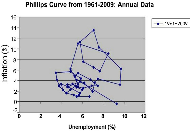
Figure 1. The annual Phillips Curve from 1961 to 2009 is “chaotic”. It appears that there is no law governing it. This chaotic pattern may be the source of confusion among economists. Our purpose is to find the general law that governs this curve. Data Source: BLS.
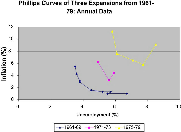
Figure 2. Without recessions, regularities of the three annual Phillips curves are recovered. Each expansion has its own Phillips curve. The 1970 and 1974 recessions shift the Phillips curve up and to the right. Tradeoff exists near the end of each of the three expansions. However, inflation and unemployment are positively related in the beginning of the two expansions 1971-1973 and 1975-1979. Data Source: BLS.
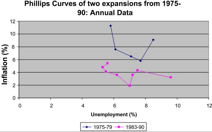
Figure 3. The 1980-1982 recession is important. It shifts the Phillips curve down and changes the tradeoff pattern. The Phillips curve for the expansion 1983-1990 has a trough in inflation around the 7 percent unemployment rate, right in the middle of that expansion. Such a case has not been observed in Figure 2. Data Source: BLS.
3. Empirical Findings
The annual and monthly graphs for 1961-1969, 1971- 1973, and 1975-1979 expansions show a clear shift pattern in the Phillips curve after each recession. The shift is up and to the right (Figures 2 and 5). The 1980-1982 recession is important. It shifts the Phillips curve downward (Figures 3 and 6). The annual Phillips curves for the second three expansions do not have a pattern as stable as the first three expansions. However, the effect of a recession on the Phillips curve is clearly shown in the graphs. The shift in the second three annual Phillips curves is in a horizontal direction from the right to the left, and the 2008 recession shifts the Phillips curve backward, from the left to the right (Figures 4 and 7). It
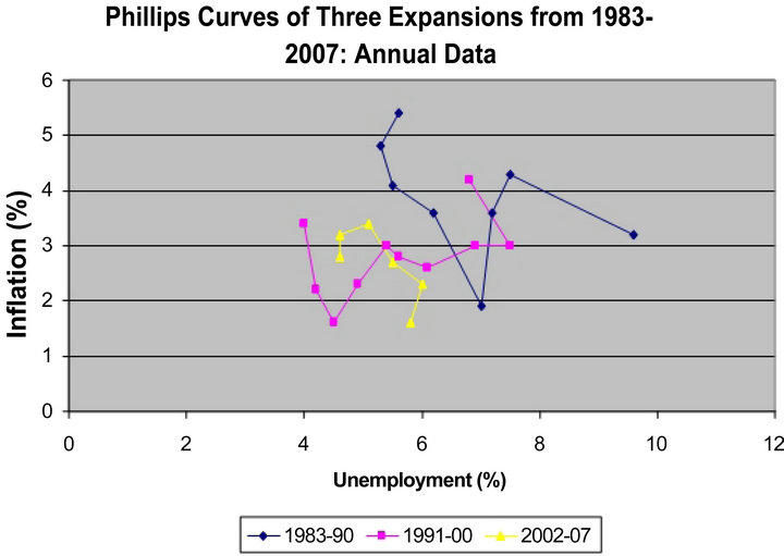
Figure 4. Each recession shifts the Phillips curve. The shift is horizontal from the right to the left, based on the initial position of each Phillips curve. Tradeoff exists near the end of each of the three expansions. Inflation and unemployment are positively related for substantial periods of time in the middle of an expansion. The decline in inflation in the middle of an expansion prolongs that expansion. Data Source: BLS.
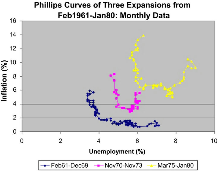
Figure 5. Inflation accelerates sharply by the end of each expansion. The inflation acceleration starts around the 4 percent unemployment rate for the 1961-1969 expansion, the 5 percent unemployment rate for the 1973-1975 expansion, and the 6 percent unemployment rate for the 1975- 1980 expansion. Inflation decelerates sharply in the beginning of each expansion, in conjunction with a decline in the unemployment rate. There are substantial periods of time in which inflation stays flat for each Phillips curve in the middle of an expansion. Data Source: BLS.
is expected that the Phillips curve after the 2008 recession will have its own pattern, which may have been affected by the Federal Reserve quantitative ease monetary policy. The inflation rate in the monthly graph for the 1961-1969 expansion stayed in a closed range between 1% and 2% when the unemployment rate was above 4% and inflation took off when the unemployment rate was about 4% (Figure 5). The acceleration in inflation was eventually stopped by the 1970 recession, induced by shocks of monetary tightening policy [15].
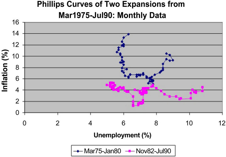
Figure 6. The 1980-1982 recession shifts the Phillips curve down and changes the tradeoff pattern considerably. The Phillips curve for the expansion from Nov 1982-Jul 1990 has a “w-shape”, with two major troughs in inflation, one tough around the 9 - 10 percent unemployment rate and the other around the 7 percent unemployment rate. Data Source: BLS.
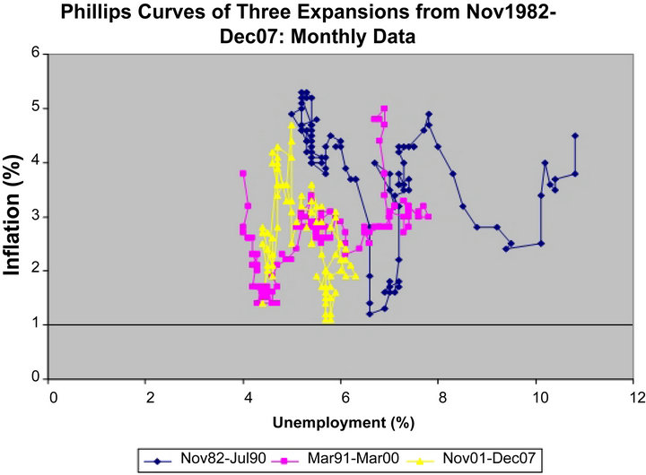
Figure 7. The Phillips cure for the 2001-2007 expansion has multiple minor “troughs” in inflation. The other two has a “w-shape” with two major troughs. The Phillips curve for the Mar91-Mar00 has one trough in inflation near the 6 percent unemployment rate and the other near the 4.5 percent unemployment rate. What is interesting is that inflation deceleration and acceleration can happen around the same unemployment rates (also see Figures 5 and 6) across expansions. Nonetheless, the 4 - 5 percent unemployment rates appear to be the key obstacle for the US economy to overcome. Data Source: BLS.
The monthly Phillips curves for the 1971-1973 and 1975-1979 expansions had a “u-shape” (Figure 5). Inflation decelerated in the beginning of each expansion to a trough, climbed out of the trough in a short period of time, stayed in a close range in the middle of that expansion, and then accelerated near the end of that expansion. The acceleration in inflation of the 1971-1973 expansion was eventually stopped by the 1974 recession, caused by oil price crisis due to OPEC [15]. The acceleration in inflation of the 1975-1979 expansion was eventually stopped by the 1980-1982 recession, induced by an oil price hike and later by a tightening monetary policy. The two ranges where inflation was flat were different. The inflation acceleration process of the 1975-1979 expansion started around the 6 percent unemployment rate. It was around this rate the inflation deceleration process of the 1971-1973 expansion started. These two expansions started with relatively high inflation and were the two shortest expansions among the six. In contrast, the 1961- 1969, 1983-1990, and 1991-1900 expansions are the three longest ones1, each of which started with a low initial inflation rate. There may be some links between the initial inflation rate when the expansion starts and the length of that expansion. The initial unemployment rate seems less important. A higher initial unemployment rate may stretch an expansion, which should be considered as good news for the current economy.
The monthly Phillips curves of the three expansions from 1983-1990, 1991-1900, and 2002-2007 had a “wshape” (Figure 7). Each of them had two or more major “troughs” in inflation with some minor ups and downs between them. The first trough was caused by the related recession. The reasons for the second or third trough were not clearly understood. The decline in inflation, after a period of acceleration, in the middle of an expansion was important in order to make that expansion continue without a recession. Moreover, the three expansions had very contained inflation rates, with average around 3 percent, close to the inflation target of the Federal Reserve after the 1980s. The decline in inflation in conjuncttion with the same in unemployment in the middle of an expansion showed that the inverse relationship between the two could fail to hold.
In summation, the monthly Phillips curve holds very well near the end of each of the six expansions. The inverse relationship between the two fails to hold in the beginning of each of the six expansions, and it may or may not hold in the middle of an expansion. The relatively steady pattern of the Phillips curve for the same expansion and the shift in the Phillips curve across different expansions show how important a recession is for the Phillips curve.
4. Inflation and Business Cycles
A business cycle is the boom and bust of an economy in its aggregate activities. No two business cycles are exactly alike; however, all business cycles are essentially alike [1,2]. Each expansion was ended by a recession induced by adverse shocks. The 2008 recession was induced by the subprime loan crises, the 2001 recession caused by the bursting of the dot-com bubble, and the 1990 recession caused by the collapsing of savings and loans, in conjunction with accounting scandals. Why do shocks matter much more when closer to the end of an economic expansion? To understand this question, and the role that a recession plays on inflation, we now provide a more detailed analysis of the inflation deceleration and acceleration around a recession. It is known in the literature that inflation is pro-cyclical with some lags [13]. What matters the most in our analysis is not the nature of the pro-cyclicality of inflation, but of the acceleration and deceleration in inflation.
Table 1 reports the case how inflation accelerates near the end of an expansion. The peaks and the left troughs are read from the monthly CPI graph created by the BLS (Figure 8). The rates of inflation at the peaks and the troughs are different across recessions. For example, the rates of inflation at the troughs range from 1.2% for the 1982-1990 expansion to 6.2% for the 1975-1980 expansion while the rates of inflation at the peaks range from 3.8% for the 1991-2001 expansion to 14.6% for the 1975-1980 expansion. The percentage increase in the rate of inflation from the inflation though to the inflation peak of a particular expansion is quite consistent and impressive. The highest percentage increase, 81%, occurred near the end of the 1982-1990 expansion. The lowest percentage increase was at 58% near the end of 1975- 1980 expansion. Thus, we find that inflation accelerated from the left inflation trough of each expansion to the inflation peak of that expansion by 58% to 81% (see Table 1 for detail), with average 68%. Inflation acceleration occurred when the labor market was tight near the end of an expansion, relative to its initial slackness when the expansion begun.
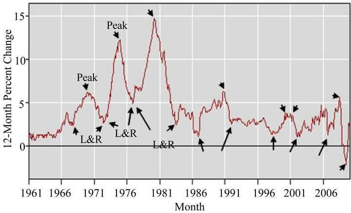
Figure 8. Monthly CPI from Jan 1961-Mar 2010. The graph was created by BLS. Arrows are added to indicate where the peaks (down arrows) and the left and right troughs (up arrows) are chosen in Tables 1 and 2. Inflation forms a “^” shape near each peak, with a recession occurring at some point between the trough and the peak of the left leg, and a recovery occurring at some point between the peak and the trough of the right leg. The right and the left legs may be uneven. Data Source: BLS.
Table 2 reports the case how inflation decelerates from the peak to its immediate (right) trough. We read the peaks and the right troughs according to the monthly CPI graph created by the BLS (Figure 8). Once again, the rates of inflation at the peaks and the right troughs are all different across recessions. For example, the rates of inflation at the right troughs range from −2.1% for the 2008 recession to 5.0% for the 1973 recession while the rates of inflation at the peaks range from 3.8% for the 2001 recession to 14.6% for the 1973 recession. The percentage decrease in the rate of inflation from the inflation peak to the inflation trough of a particular recession is equally impressive, from 138% of the 2008 recession to 55% of the 1969 recession. The highest percentage decrease, 138%, occurred during the 2008 Great Recession. In summation, we find that inflation decelerated from the peak to its immediate trough (see Table 2 for detail) by 55% to 138%, with average decrease at 75%.
We also find that inflation acceleration or deceleration could happen in the middle of an expansion as well. Moreover, any such inflation acceleration was accompanied by a deceleration as that expansion proceeded.
Inflation acceleration at the end of an expansion reduces the purchasing power of dollars as well as the real balance of money supply. A decline in the former reduces personal and public consumption while a decline in the later likely raises the real interest rate at equilibrium [13]. With higher real and nominal interest rates, private investment declines. Thus, a sharp rise in the inflation rate can substantially weaken the economy and make it more fragile to adverse shocks. This provides a reasonable explanation why adverse shocks matter much more near the end of an expansion. In contrast, a sharp deceleration in inflation plays the opposite role and helps the economy recover from a recession.
Inflation acceleration and deceleration is the outcome of an integration process of human behaviors in a business cycle under a given market system. For a fifty years time span for the US economy, both population and labor forces have substantially increased, and old generations have been replaced by new generations. Furthermore, technology in production has advanced considerably. Internets and online businesses which play so important role for today’s economy did not even exist in the 60s and 70s. The “true” economic structure may indeed have changed to a great extent during this period of time. However, some basics remain. Human behaviors, as revealed in Tables 1 and 2, are essentially alike, despite substantial differences exist among the six recessions and recoveries. Economics should be a science that aims at finding such regularities in human behaviors under a given market institution. Although economic structures may change across time, human behaviors may stay the same.
5. Monetary Policy
The very value of the Phillips curve for conducting monetary policy is not seen during the periods when the economy is in a recession. There are fewer debates as to what the Federal Reserve should do during a recession. After the economy has expanded for a substantial duration, economists often disagree with each other as to what the Federal Reserve should or should not do. The Phillips curve holds true near the end of each of the six expansions we have studied. This implies that the Phillips curve should remain as a useful tool for the Federal Reserve to conduct its policy, only after an expansion has lasted for a substantial period of time.
In addition, the Federal Reserve should carefully watch the time when inflation reaches its peaks and troughs and then conduct the monetary policy accordingly. When inflation climbs from a lower level trough with a slack labor market up to a certain high level, a tightening monetary policy should be used to keep inflation near a target. When inflation climbs up from a lower level trough with a tight labor market, the Federal Reserve should use a tightening policy with caution. It is right at this point that there is a dilemma in conducting a monetary policy. An aggressive tightening may create shocks and bring the economy into a recession. But the inflation pressure built in during the expansion requires such a policy to keeping inflation in control. There is no perfect solution to this dilemma. Because the inflation acceleration reduces the real balance of money supply, a tightening policy at the moment, as often implemented in the past, will decrease the real balance of money supply even more. This will sharply reduce personal consumption and private investment because of a higher real interest rate at equilibrium. Our suggestion is to do the opposite: Use a moderately ease monetary policy because we know that a recession will be on its way. Inflation will eventually decelerate after a recession actually occurs. An ease monetary policy will reduce the pain caused by the decline in the real balance of money supply due to acceleration in inflation. Such a policy is likely to moderate the recession that will follow.
Our observations show that an expansion will eventually end up with inflation acceleration, which in turn will be stopped by a recession. Thus, monetary policy should not aim at elimination of recessions. A recession is the best friend to the Federal Reserve in its battle against inflation. What the Federal Reserve should pay attention to is the trough in inflation when the acceleration starts. This trough will affect the peak and then the next trough after the recession (Tables 1 and 2).
6. Open Questions
We raise two open questions about unemployment and business cycles. What causes the acceleration in inflation near the end of an expansion? An answer to the question must have something to do with the expansion itself and the related new hiring of employees. This raises another important question: If it is the expansion that accelerates inflation, which in turn makes the economy fragile to adverse shocks, why cannot firms forgo hiring freezes and kill a recession at bay?
The rate of unemployment in the US economy from 1961-2010 had very low volatility in its uptrend and downtrend during each business cycle, unlike the inflation rate. Once it was in a downtrend (uptrend), only a recession (recovery) made it turn upward (downward) for a substantial duration. It appears that when the US economy starts to generate (destruct) net numbers of jobs, it rarely stops before a recession (recovery). What makes the labor market function this way? These two questions may be closely related to the question what are the general laws that govern business cycles in capitalist economies raised by Robert Lucas [2].
7. Discussion
It is a recession that turns the rate of unemployment from a downtrend into an uptrend, and it is a recession that eventually turns an uptrend in inflation near the end of an expansion into a downtrend (Figure 8). A recession not only shifts the Phillips curve but also changes its pattern. The fact that inflation acceleration and deceleration can happen at the same level of unemployment rates across different business cycles shows why it is important to treat each business cycle separately in order to study the Phillips curve. A study of the Phillips curve by gathering data of two business cycles in the same economy is like to put two different kinds of fruits into one single basket. Useful information about how an economy may operate is lost in such a study, for it does not provide an accurate picture how inflation and unemployment actually perform during an expansion or a contraction. This also casts a doubt of an attempt that aims at the inverse relationship between the average rates of inflation and unemployment across different business cycles, an approach pioneered by A. W. Phillips [3]. In that sense, the methodology in A.W. Phillips [3] may be wrong when it is applied to the US data. Such an error in methodology in the study for the US economy can be a potential source of confusion among economists (Figure 1). Nevertheless, his finding of the tradeoff holds true near the end of each of the six expansions we have studied. Such a tradeoff may well exist for the future business cycles of the US economy. In this sense, his finding is quite magnificent and useful for the monetary policy of the Federal Reserve.
8. Acknowledgements
I thank an anonymous referee and my colleague I-Ming Chiu for their comments that help improve the paper.
REFERENCES
- G. W. Stadler, “Real Business Cycles,” Journal of Economics Literature, Vol. XXXII, 1994, pp. 1750-1783.
- R. E. Lucas, “Studies in Business Cycle Theory,” The MIT Press, Cambridge, 1981.
- A. W. Phillips, “The Relation between Unemployment and the Rate of Change of Money Wage Rates in the United Kingdom, 1861-1957,” Economica, Vol. 25, No. 100, 1958, pp. 283-299.
- R. G. King and M. W. Watson, “The Post-War US Phillips Curve: A Revisionist Econometric History,” Carnegie-Rochester Conference Series on Public Policy, Vol. 41, No. 1, 1994, pp. 157-219.
- P. A. Samuelson and R. M. Solow, “Analytical Aspects of Anti-Inflation Policy,” American Economic Review, Vol. 50, No. 2, 1960, pp. 177-194.
- M. Friedman, “The Role of Monetary Policy,” American Economic Review, Vol. 58, No. 1, 1968, pp. 1-17.
- E. S. Phelps, “Phillips Curves, Expectations of Inflation and Optimal Unemployment over Time,” Economica, Vol. 34, No. 135, 1967, pp. 254-281. doi:10.2307/2552025
- E. S. Phelps, “Money-Wage Dynamics and Labor-Market Equilibrium,” Journal of Political Economy, Vol. 76, No. 4, 1968, pp. 678-711. doi:10.1086/259438
- J. Galı́ and M. Gertler, “Inflation Dynamics: A Structural Econometric Analysis,” Journal of Monetary Economics, Vol. 44, No. 2, 1999, pp. 195-222. doi:10.1016/S0304-3932(99)00023-9
- F. Schorfheide, “DSGE Model-Based Estimation of the New Keynesian Phillips Curve,” Economic Quarterly, Vol. 94, No. 4, 2008, pp. 397-433.
- G. Calvo, “Staggered Prices in a Utility-Maximizing Framework,” Journal of Monetary Economics, Vol. 12, No. 3, 1983, pp. 383-398. doi:10.1016/0304-3932(83)90060-0
- R. E. Lucas, “Econometric Policy Evaluation: A Critique,” Carnegie-Rochester Conference Series on Public Policy, Vol. 1, No. 1, 1976, pp. 19-46. doi:10.1016/S0167-2231(76)80003-6
- O. Blanchard, “Macroeconomics,” Prentice Hall, Upper Saddle River, 1997.
- K. E. Case, R. C. Fair and S. M. Oster, “Principles of Macroeconomics,” 9th Edition, Prentice Hall, Upper Saddle River, 2008.
- P. Temin. “The Causes of American Business Cycles: An Essay in Economic Historiography,” NBER working paper series, Cambridge, 1998.
NOTES
1We see the 1980 and 1982 NBER recessions as one recession instead of two, following popular text books [13,14].