Modern Economy
Vol. 4 No. 5 (2013) , Article ID: 32368 , 17 pages DOI:10.4236/me.2013.45036
Econographication
Faculty of Economics and Administration, University of Malaya, Kuala Lumpur, Malaysia
Email: marioruiz@um.edu.my
Copyright © 2013 Mario Arturo Ruiz Estrada. This is an open access article distributed under the Creative Commons Attribution License, which permits unrestricted use, distribution, and reproduction in any medium, provided the original work is properly cited.
Received February 8, 2011; revised March 8, 2013; accepted April 8, 2013
Keywords: Graphs in Economics; Economics Teaching; Multidimensional Graphical Modeling
ABSTRACT
The rationale of Econographication revolves around the efficacy of multidimensional graphs as the most effective visual tool to understand any economic phenomenon from a multidimensional view. The main motivation behind the creation of Econographication is to evaluate multidimensional graphs evolved so far in economics and to develop new type of multidimensional graphs to facilitate the study of economics, as well as finance and business. Thereby, the mission of Econographication is to offer academics, researchers and policy maker’s an alternative multidimensional graphical modeling approach to the research and teaching-learning process of economics, finance and business from a multidimensional perspective. Hence, this alternative multidimensional graphical modeling approach is offering a set of multidimensional coordinate spaces to build different types of multidimensional graphs to study any economic phenomenon. The following new types of multi-dimensional coordinate spaces are presented: the pyramid coordinate space (five axes and infinite axes); the diamond coordinate space(ten axes and infinite axes); the 4-dimensional coordinate space (vertical position and horizontal position); the 5-dimensional coordinate space (vertical position and horizontal position); the infinity-dimensional coordinate space (general approach and specific approach); the inter-linkage coordinate space; the cube-wrap coordinate space; the mega-surface coordinate space. All these multi-dimensional coordinate spaces mentioned previously, they are available to represent graphically 4-dimensions, 5-dimensions, 8-dimensions, 9-dimensions until infinity-dimensions.
1. The Evolution of Graphical Methods in Economics
Research leading to this chapter shows a strong link between the introduction of graphical methods in economics and the development of theories, methods and techniques in statistics and mathematics. In the 18th century, for example, several new graphical methods were developed as a result of some mathematics and statistics research in the same century. These graphical methods include line graphs of time series data (since 1724), curve-fitting and interpolation (1760), measurement of error as a deviation from the graphed line (1765), graphical analysis of periodic variation (1779), a statistical mapping (1782), bar charts (1756) and printed coordinate chapter (1794) [1].
The application of graphical methods in the economic analysis, we have renowned economists like William Playfair [2], Francis Ysidro Edgeworth [3] and William Stanley Jevons [4]. According to Harro Maas [5], William Playfair constructed a wonderful collection of plates and graphs at the end of the eighteenth century. In his book entitled Commercial and Political Atlas, Playfair focused on the study of trade cycles. This placed him far ahead of other economists at the time in terms of visualizing socio-economic data. We would classify the development of the usage of graphical methods in economics into two phases. The first phase is the descriptive graphical method. It is supported by simple tables, histograms, line graphs and scatter-plots. All these types of graphs are based on the visualization of a single economic variable (vertical axis = Y) through a specific period of time (horizontal axis = X) in the first quadrant in the 2-dimensional Cartesian coordinate system is shown in Figure 1.
The main objective of the descriptive graphical method in economics is to study the behavior of a single economic variable (e.g. exports, imports, unemployment, GDP, inflation rate etc.) within a time frame (per decade, annually, monthly, weekly or daily) based on time-series. In fact, William Playfair may be considered the pioneer and promoter of the descriptive graphical method.
The second phase in the development of graphical methods for economics will be called the “analytical
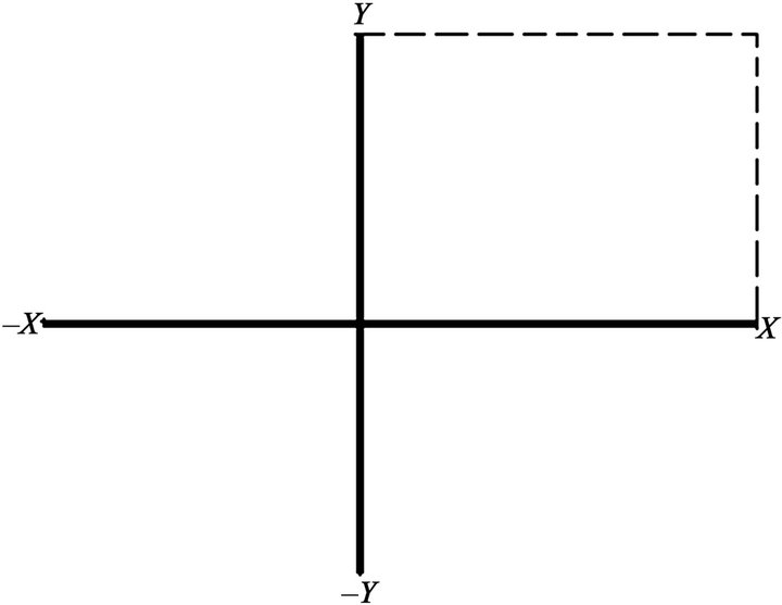
Figure 1. 2-Dimensional coordinate space.
graphical method”. The analytical graphical method in economics features by 2-dimesnional and 3-dimensional coordinate systems. According to Harro Maas is William Stanley Jevons who first explored the merits of the graphical method for political economy. Jevons did this through the function called “King-Devenant Law of Demand” that he introduced. This is a case of the use of analytical graphical method in economics, where the form of the graph gives an idea of the possible class of the functions describing the relationship between X and Y variables respectively that suggest a causal interpretation of the relationship between X and Y.
Additionally, we like to mention also that the uses of the formal graphical method based on the 2-dimensional Cartesian plane was introduced in 1637 by René Descartes [6], whose contributions to different scientific disciplines, of which economics was one, were substantial. The 2-dimensional coordinate space opened a new era in economic analysis by providing for analysis of a single economic phenomenon based on the relationship between two variables.
However, it is necessary to mention the major contribution of Antoine Augustin Cournot [7]. Cournot derived the first formula for the rule of supply and demand as a function of price on 2-dimensional view. He was, in fact, also the first economist to draw the supply and demand curves on a graph. Cournot believed that economists must utilize graphs only to establish probable limits and express less stable facts in more absolute terms. He further held that the practical use of mathematics in economics involves not only strict numerical precision, but also graphical visualization. Besides Cournot and Jevons, other innovator economists that contributed to the analytical graph system in economics over time are Leon Walras (with general equilibrium), Alfred Marshall (with partial equilibrium) and Joseph Schumpeter (with business cycles) [8].
In the 20th century the use and application of the analytical graphical method among economists were often based on sophisticated mathematical and graphical techniques introduced during the development of new economic models. In particular, calculus, trigonometry, geometry and statistical and forecasting methods started to be employed by economists in constructing their graphs during that time. In addition, 2-dimensional and 3-dimensional Cartesian coordinate systems were also a part of complex economics research Avondo-Bodino [9]. Consequently, the application of sophisticated mathematical and graphical techniques can be seen in the development of the following economic models and theories: welfare theory [10], IS-LM curve (Hansen, 1938) [11], development of static and dynamic analysis [12], econometrics [13], Phillips curve [14], Okun law [15], economic growth theory [16], game theory [17], introduction of dynamic models and econometrics [18], monetary theory [19], and rational expectations theory [20].
The rapid development of the analytical graphical method has been facilitated by high technology and sophisticated analysis instruments such as the electronic calculator and the computer. The development of analysis instruments in economics took place into two stages. The first stage involved the “basic computational instruments”, where electronic calculators were used to compute basic mathematical expressions (e.g. long arithmetic operations, logarithm, exponents and squares). This took place between the 1950’s and 1960’s. The second stage called “advance computational instruments” took place in the middle of the 1980’s. This is when high speed and storage-capacity computers using sophisticated software were introduced for the first time. The use of sophisticated software enables easy information management, application of difficult simulations as well as the creation of high resolution graphs under 3-dimensional coordinate system. The analysis instruments undoubtedly contributed substantially to the development and research in economics.
Therefore, high computational instruments, backed by sophisticated hardware and software, are utilized to create graphical representations with high resolution and accuracy. In fact, the descriptive graphical method and analytical graphical method can be categorized according to functions or dimensional. In terms of function, these two graphical methods are either descriptive or analytical. In terms of dimension, these two graphical methods can be either 2-dimensional, 3-dimensional and multi-dimensional coordinates systems. The descriptive graphical method shows arbitrary information that is used to observe the historical data behavior from a simple perspective. On the other hand, the analytical graphical method is available to generate time-series graphs, cross-section graphs and scatter diagrams to show the trends and relationships between two or more variables from a multi-dimensional and dynamic perspective.
2. A Short Review about Dimension and Coordinate Systems (Cartesian Plane and Coordinate Space)
Initially, we like to review four basic definitions about dimension. According to the first definition about dimension by Poincarė [21], he defines dimension as a space that is divided by a large number of sub-spaces. It meant “however we please” and “partitioned”. The second definition about dimension is given by Brouwer [22]. He defines dimension as “between any two disjoint compacta”. Brouwer makes references about the existence of a group of sub-sets into different sets. It is based on the uses of the topological dimension of a compact metric space based on the concept of cuts [23]. The third definition about dimension is given by Urysohn and Menger [24], they defined dimension as “between any compactum and a point not belonging to it”. These four authors are sharing common concepts into its definitions about dimension such as the uses of spaces, subspaces, sets, subsets, partitioned and cut concepts. This mean that any dimension needs to be studied by spaces/sets or subspaces/sub-sets or partitioned/cuts.
The idea about dimension is complex and deeper for the human mind. It is because we need to do often abstractions and parameterizations of time and space of any geometrical object that cannot be visualized in the real world [25]. Moreover, this part of our research is interested to propose an alternative definition about dimension. According to this book “dimension” can be defined “as the unique mega-space that is build by infinite general-spaces, sub-spaces and micro-spaces that are interconnected systematically.” In the process to visualize different dimensions graphically, it is possible by the uses of coordinate systems. The coordinate systems are available to generate the graphical modeling frameworks to represent different dimension(s) in the same graphical space. The coordinate systems can be divided by two types: Cartesian plane and coordinate space.
The difference between the Cartesian plane and coordinate space is originated by the number of axes. In the case of the Cartesian plane is based on the uses of two axes and the coordinate space is based on the uses of three or more axes. Therefore, the Cartesian plane and coordinate space are available to generate an idea about dimension(s) graphically through the optical visualization of several lines in a logic order by length, width and height. The concept about dimension also can be explained by the Euclidian geometry under the uses of the Euclidian spaces. The Euclidian geometry can be divided by the 2-dimensional Euclidean geometry (plane geometry) and the 3- dimensional Euclidean geometry (solid geometry). Additionally, the study of the Euclidian geometry also involves the study of the n-dimensional space represented by Rn or En under the uses if the n-dimensional space and n-vectors respectively.
3. How Multi-Dimensional Coordinate Spaces Work?
The main reason to apply multi-dimensional coordinate spaces is to study any economic phenomena from a multidimensional perspective. It is originated by the limitations that the 2-dimensional coordinate space shows in the moment to generate a multidimensional optical visual effect of any economic phenomena at the same graphical space. Hence, the multidimensional coordinate spaces leads an alternative graphical modeling more flexible and innovative than the 2-dimensional coordinate space in the moment to observe multi-variable data behavior.
The study of multi-dimensional coordinate spaces requests basic knowledge about the “n-dimensional space”. The idea about the n-dimensional space was originated by many Greeks thinkers and philosophers such as Socrates, Plato, Aristotle, Heraclitus and Euclid (father of the geometry). The great contribution of Euclid in geometry was the design of the plane geometry under the 2-dimensional Euclidean geometry and the solid geometry under the 3-dimensional Euclidean geometry. However, the n-dimensional space can be defined as a mental refraction through the optical visualization and brain stimulation by several lines in a logic order by length, width, height and colors to represent the behavior of simple or complex phenomena in different periods of time in the same graphical space.
Usually, the study of n-dimensional space is based on the application of the “coordinate system“. In fact, the coordinate spaces can be classified by 2-dimensional coordinate space, 3-dimensional coordinate space and multidimensional coordinate spaces. The main role of coordinate system is crucial in the analysis of the relationship between two or more variables such as exogenous variable(s) and endogenous variable(s) on the same graphical space. In fact, the Euclidean space is given only the mathematical theoretical framework, but not the graphical modeling to visualize the n-dimensions according to different mathematical theoretical research works. On the other hand, Minkowski’s [26] introduce the idea about the 4-dimensional space or the “world”. The world according to Minkowski’s it is originated by the application of 3-dimensional continuum (or space). The difference between the 4-dimensional space and 3-dimensional space graphical model is that the first graphical model replace (X,Y,Z) by (X1,X2,X3,X4), thus X1 = X; X2 = Y; X3 = Z and X4 = . The X4 is based on the application of the Lorenz transformation axiom. The 4-dimensional space by Minkowski’s also never offer a specific graphical modeling or alternative Cartesian coordinate system to help visualize the 4-dimensional space, it is only offer a mathematical theoretical framework to describe the idea about 4-dimensional space. Moreover, the application of multi-dimensional coordinate spaces offer a large possibilities to adapt n-dimensions, sub-dimensions, microdimensions, nano-dimensions and ji-dimensions in the visualization of any economic phenomenon.
Basically, the uses of coordinate spaces by economists are based on plot different dots that represent the relationship between two or more variables (endogenous and exogenous) in the first and fourth quadrants in the 2- dimensional coordinate space. After, they proceed to join all these dots by straights lines until is possible to visualize histograms, line graphs and scatter-plots are shown in Figures 1 and 2. Hence, it is possible to observe the trend and behavior of different variables of any economic phenomenon. For example, the relationship between unemployment/inflation, interest-rate/investment, prices/quantity demand and supply, etc.
From our point of view, each dot is plotted on the 2- dimensional, 3-dimensional and multi-dimensional coordinate spaces represent a single rigid point. In fact, the plotting of a single rigid point in any coordinate space requests the application of two basic assumptions: first assumption is that two rigid points cannot occupy the same space at the same time. The second assumption is that different rigid point(s) deal in different n-dimensional spaces is moving under different speeds of time. The variable “time” in the case of multi-dimensional coordinate spaces needs to be classified by: the general time, partial time and constant time. The general time is running in the general-space but in the case of the subspaces, micro-spaces, nano-spaces are running under different partial times. In the case of JI-spaces always is fixed by the constant time. Recently, few economists start to use the 3-dimensional coordinate space in economics by the uses of three axes: “X-coordinate” (or exogenous variable), “Y-coordinate” (or exogenous variable) and the “Z-coordinate” (or endogenous variable). It is based on the construction of surfaces or 3-dimensional manifolds to visualize multi-variable economic data behavior are shown in Figure 2. According to our research the uses of the 3-dimensional coordinate space are not so popular among economists and policy makers.
Based on one thousand five hundred (1500) chapters published in twenty one (21) reputable economics journals1 between the year 1939 and 2009 [27], it is possible
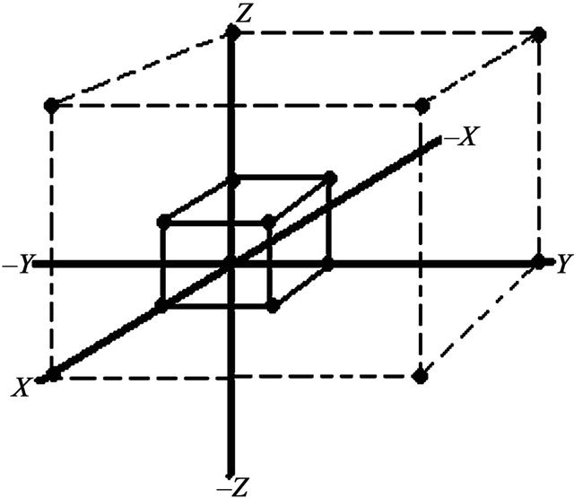
Figure 2. 3-Dimensional coordinate space.
to observe that the common types of graphical representations applied in the study of social sciences, especially in economics, were of the 2-dimensional coordinate spaces. It is according to 99.5% of these chapters applied 2-dimensional Cartesian coordinate system, and only 0.5% of them applied 3-dimensional coordinate spaces. Additionally, this research will find some reasons about “why” economists continue using 2-dimensional coordinate space or sometimes 3-dimensional coordinate space in the graphical representation of complex and dynamic economic phenomena, these reasons are following by:
● The 2-dimensional graphical models are established for long time, since the introduction of the 2-dimensional coordinate space by Descartes until today. The application of 2-dimensional coordinate space in the economic graphical analysis became by “Tradition”.
● The 2-dimensional space is “easy to apply” to visualize basic trends or values in the same graphical space. The logic explanation about the common uses of the 2-dimensional coordinate space, it can be originated by the easy way to plot, draw and visualize any economic phenomenon. Therefore, 2-dimensional coordinate space can generate a clear visual and mental refraction to understand complex and dynamic economic phenomena graphically in the same space and time.
Difficulty to find “alternative and suitable multidimensional graphical models” to generate the transition from 2-dimensional coordinate space graphical modeling to multi-dimensional spaces graphical modeling. This research found some difficulties to generate this crucial visual and mental transition from 2-dimensional coordinate space to multi-dimensional coordinate space. It can be originated by some difficulties in the process to plot, draw and visualization of multi-dimensional graphs.
Finally, a new set of multi-dimensional coordinate spaces is introduced in this document. The idea is to generate a new multidimensional optical visual effect to visualize complex economic phenomena. We can observe that into the multidimensional coordinate spaces can keep a large number of exogenous variables that are changing constantly and affect directly on the endogenous variable(s) behavior in the same graphical space. These new type of multi-dimensional coordinate spaces are based on the pyramid coordinate space (five axes and infinite axes), the diamond coordinate space(ten axes and infinite axes), the 4-dimensional coordinate space (vertical position and horizontal position), the 5-dimensional coordinate space (vertical position and horizontal position), the infinitedimensional coordinate space (general approach and specific approach), the inter-linkage coordinate space, the cubewrap coordinate space, and the mega-surface coordinate space. Being multi-dimensional, it enables economists, academics and policy makers to analyze economic phenomena from multidimensional perspectives across time and space.
4. An Introduction to Omnia Mobilis Assumption
Basically, the idea to build an economic model is to simplify the real economic world. It is based on the uses of a large number of variables that interacting together into the same economic phenomenon. To analyze an economic phenomenon can be by induction (particular observations) or deduction (simple forecasting). According to our research, any economic model will try to show the interaction of different economic actors and different possible scenarios. The main problem is how to catch-up the dynamic changes across time (period of time in analysis) and space (geographical place in analysis) in any economic model as a whole.
For long time economists and academics are applied the Ceteris Paribus assumption to build economic models. Especially in old economic models such as demand and supply model that explain basically the relationship between two variables: endogenous variable (quantity) and exogenous variable (price) into a precise period of time and space. In other words, we leave the rest of variables out currently until we can get the final result from these two specific variables in analysis.
The Ceteris Paribus assumption also can be considered the most common assumption that is learned and applied by economists to understand different economic phenomena. This assumption translated from Latin that it means “all other things [being] the same”. It facilitates the description of how a variable of interest changes in response to changes in other variables by examining the effect of one variable at a time. An extremely important contribution of Alfred Marshall, it supports the understanding of the application of Ceteris Paribus assumption in economic models. According to Marshall [28]:
“The element of time is a chief cause of those difficulties in economic investigations which make it necessary for man with his limited powers to go step by step; breaking up a complex question, studying one bit at a time, and at last combining his partial solutions into a more or less complete solution of the whole riddle. In breaking it up, he segregates those disturbing causes, whose wanderings happen to be inconvenient, for the time in a pound called Ceteris Paribus. The study of some group of tendencies is isolated by the assumption other things being equal: the existence of other tendencies is not denied, but their disturbing effect is neglected for a time. The more the issue is thus narrowed, the more exactly can it be handled: but also the less closely does it correspond to real life. Each exact and firm handling of a narrow issue, however, helps towards treating broader issues, in which that narrow issue is contained, more exactly than would otherwise have been possible.”
Marshall’s approach thus allows the analyses of complex economic phenomena by parts where each part of the economic model can be joined to generate an approximation of the real world. This approach can be termed the Isolation Approach and according to Marshall [29] originates from two possible isolation clauses. First the Ceteris Paribus assumption allows some variables to be considered unimportant. This clause is called Substantive Isolation.
The Substantive Isolation considers that some unimportant variables cannot significantly affect the final result of the economic model. Second, the Ceteris Paribus assumption allows the influence of some important factors to be disregarded. The application of the Ceteris Paribus assumption in this case is purely hypothetical; therefore the second clause is called Hypothetical Isolation. It allows parts of the model to be managed more easily.
In other words, to explain a complex economic phenomenon, the Ceteris Paribus approach considers the effect partially of each variable in a set of m variables (termed usually independent variables, Xj , j = 1, 2, ... , m) upon a variable of interest (usually termed the dependent variable, Y). From a mathematical point of view, the Ceteris Paribus assumption in an economic model is equivalent to the partial derivative, which explains how one exogenous variable, say Xk, in a set of exogenous variables can affect directly on the endogenous variable Y while the other exogenous variables are being held constant. From a graphical point of view, the Ceteris Paribus assumption supports the elaboration of scenarios that can be visualized on 2-dimensional coordinate space.
More precisely, if “Y” is a function of, say, X1 and X2, the (partial) relationship between Y and X1 can be visualized in the 2-dimensional space describing Y and X1,
assuming X2 is held constant. In order to approximate real world, Marshall goes on to propose that “With each step more things can be let out of the pound; exact discussions can be made less abstract, realistic discussions can be made less inexact than was possible at an earlier stage.” The real-world scenario is thus approximated by the cumulative effect of the partial effects of the X variables on Y. After our review about the Ceteris Paribus assumption, according to our research we find that part of the problem to suggest the application of Ceteris Paribus assumption can be originated by three basic reasons follow by:
● First reason is the historical momentum that this assumption was build to help explain a economic phenomenon, maybe the number of variables are accounted was less before than in our days.
● Second reason is that the Ceteris Paribus assumption can be considered the basic and classic tool for teaching-learning economics.
● Third reason is from the graphical modeling, it is based on the application of 2-dimensional coordinate space (X,Y) that is used for long time. According to our research the 2-dimensional coordinate space is not available to visualize multi-variable economic modeling into the same graphical space. Thereby, the 2-dimensional coordinate space is only available to visualize two variables: endogenous variable and exogenous variable simultaneously into the same graphical space.
The idea to introduce the Omnia Mobilis assumption—everything is moving—[30] is to reduce the dependency and less uses of Ceteris Paribus assumption in the economic modeling. We propose the openness of substantive isolation through the application of the Omnia Mobilis assumption. It is based on generate the relaxation of all variables without restrictions and limitation that the Ceteris Paribus assumption generates into the economic modeling. To generate this relaxation of a large number of variables in any economic modeling, we suggest the application of multi-dimensional coordinate spaces that is offer by Econographication [31]. The idea is to draw multidimensional graphs can help in the visualization all changes of several numbers of variables in the same graphical space. Additionally, the multidimensional graphs provide an alternative graphical approach to the Marshall view of step-by-step cumulative partial approach to the economic modeling. The main objective to apply multidimensional graphs is to visualize graphically all changes of the endogenous variable in response to the changes of several numbers of exogenous variables simultaneously. The multidimensional graphs can also be used to show the dynamic behavior of different variables in any economic model without any restriction. The application if the Omnia Mobilis assumption is to capture all possible economic actors and different possible scenarios into the same picture. Therefore, this chapter proposes that Ceteris Paribus assumption is not necessary to be used when economists have opportunity to use the Omnia Mobilis assumption and multidimensional graphs.
The Omnia Mobilis assumption also suggests the application of economic modeling in real time to observe the changes of all variables in real time. It is to demonstrate that the economic modeling don’t request the application of Ceteris Paribus assumption in the study of dynamic and complex economic phenomenon, because according to our research any economic phenomenon always still alive and never keep a constant behavior. The difference between Ceteris Paribus assumption and Omnia Mobilis assumption is that the Ceteris Paribus assumption only takes a photo just into a specific historical momentum of some economic phenomenon, but in the case of Omnia Mobilis assumption show a video that is running in real time. Moreover, the multidimensional graphs play a crucial role to understand the application of the Omnia Mobilis assumption in the economic modeling. In fact, the multidimensional graphs are available to visualize the changes of all exogenous variables simultaneously can affect on a single variable or endogenous variable in the same time and space. Finally, the Omnia Mobilis assumption opens a new era in the economic modeling under the application of multidimensional graphs and economic modeling in real time. We can say that the contribution of the Ceteris Paribus assumption in the economic modeling was great at the past, but in our days this assumption is not enough to explain the complexity and dynamicity of different economic phenomena as a whole.
5. The Classification of Multi-Dimensional Coordinate Space
The multi-dimensional coordinate spaces [32] can be classified by the pyramid coordinate space (five axes and infinite axes), the diamond coordinate space(ten axes and infinite axes), the 4-dimensional coordinate space (vertical position and horizontal position), the 5-dimensional coordinate space (vertical position and horizontal position), the infinity-dimensional coordinate space (general approach and specific approach), the inter-linkage coordinate space, the cube-wrap coordinate space, and the megasurface coordinate space.
5.1. The Pyramidal Coordinate Space with Five Axes
The pyramidal coordinate space with five axes consist in four independent axes (X1, X2, X3, X4) and one dependent axis (Y*). The Y* axis is positioned in the center part of this coordinate space among of the other four axes: X1, X2, X3, X4. The function used by the pyramidal coordinate space with five axes is fixed by Y* = ƒ(X1, X2, X3, X4), where X1, X2, X3, X4, Y* axes are using only real positive numbers R+ under the condition 0 ≥ R+ ≤ + ∞. The only uses of positive axes in the pyramidal coordinate space with five axes request the uses of absolute values. The uses of absolute values in each axis are based on the application of the non-negative property.
Hence, all axes |X1|, |X2|, |X3|, |X4|, |Y*| always use values large or equal than zero. The pyramidal coordinate space with five axes show clearly into the same graphical space any possible change(s) of any or all values plotted on each or all X1, X2, X3, X4 axes that can affect directly on the behavior of Y* axis value. In order to plot different values in each axis into the pyramidal coordinate space with five axes, we need to plot each value directly on its axis line. At the same time, all values were plotted on each axis line need to be joined together by straight lines until we can visualize a pyramid-shaped figure with five faces are shown in Figure 3. Therefore, we have two possible graphical scenarios: first graphical scenario, if all or any X1, X2, X3, X4 axes values move from outside to inside, then Y* axis value move down. Second graphical scenario, if all or any X1, X2, X3, X4 axes values move from inside to outside, then Y* axis value move up. Basically, the pyramidal coordinate system with five axes is represented by:
([X1, X2, X3, X4], Y*) (1)
5.2. The Pyramidal Coordinate Space with Infinite Axes
The pyramidal coordinate space with infinite axes consist in infinite independent axes (X1, X2, X3,…,X∞) and one dependent axis (Y*). The Y* axis is positioned in the center part of this coordinate space among of the other infinite axes: X1, X2, X3,…, X∞. The function used by the pyramidal coordinate space with infinite axes is fixed by Y* = ƒ(X1, X2, X3,…, X∞), where X1, X2, X3,…, X∞, Y* axes are using only real positive numbers R+ under the condition 0 ≥ R+ ≤ + ∞.
The only uses of positive axes in the pyramidal coordinate space with infinite axes request the uses of abso-
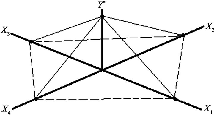
Figure 3. Pyramid coordinate space.
lute values. The uses of absolute values in each axis are based on the application of the non-negative property. Hence, all axes |X1|, |X2|, |X3|, |X4|, |Y*| always use values large or equal than zero. The pyramidal coordinate space with infinite axes show clearly into the same graphical space any possible change(s) of any or all values plotted on each or all X1, X2, X3,…, X∞ axes that can affect directly on the behavior of Y* axis value.
In order to plot different values in each axis into the pyramidal coordinate space with infinite axes, we need to plot each value directly on its axis line. At the same time, all values were plotted on each axis line need to be joined together by straight lines until we can build a pyramidshaped figure with infinite faces are shown in Figure 4.
Therefore, we have two possible graphical scenarios: first graphical scenario, if all or any X1, X2, X3,…, X∞ axes values move from outside to inside, then Y* axis value move down. Second graphical scenario, if all or any X1, X2, X3,…, X∞ axes values move from inside to outside, then Y* axis value move up. The pyramidal coordinate system with infinite axes is represented by:
([X1, X2, X3,…, X∞], Y*) (2)
5.3. The Diamond Coordinate Space with Ten Axes
The diamond coordinate space with ten axes has two levels of analysis and ten axes. Each level of analysis is represented by (XL:i, YL:i ), where “L” represents the level of analysis, in this case either level one (L1) or level two (L2); “i” represents the quadrant level of analysis (in this case, quadrant 1, 2, 3 or 4). In order to plot different values in each axis into the diamond coordinate space with ten axes, we need to plot each value directly on its axis line respectively. At the same time, all values were plotted on each axis line need to be joined together by straight lines until we can build a diamond-shaped figure with eight faces are shown in Figure 5. It is important to mention at this juncture that the first level (L1) has five axes represented by X1:1, X1:2, X1:3, X1:4, Y1. Four independent axes represented by X1:1, X1:2, X1:3, X1:4 and one dependent axis fixed by Y1 respectively. The second level (L2) has five axes represented by X2:1, X2:2, X2:3, X2:4, Y2. We assume that does not exists any relationship between
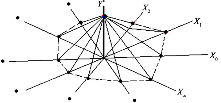
Figure 4. The pyramid coordinate space with infinite axes.
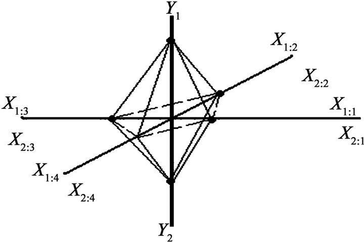
Figure 5. Diamond coordinate space.
level one (L1) and level two (L2) of analysis. The common issue between these two levels of analysis is that both levels use the same XL:i axes in the diamond coordinate space. However, level one (L1) of the analysis cannot affect level two (L2) of the analysis, and vice versa. If we draw different levels of analysis in the diamond coordinate space, we can visualize and compare two different scenarios in the same diamond coordinate space at the same time is shown in Figure 5. It is crucial to mention at this point that the fifth and tenth axes (Y1 and Y2) is positioned in the center part of the diamond coordinate space among the other eight axes: X1:1, X1:2, X1:3, X1:4, X2:1, X2:2, X2:3, X2:4.
We assume that both YL (Y1, Y2) use only real positive numbers R+. Therefore, the diamond coordinate space all X1:1, X1:2, X1:3, X1:4, Y1, X2:1, X2:2, X2:3, X2:4, Y2 axes are either on the positive side of respective axes together. The only uses of positive axes in the diamond coordinate space request the uses of absolute values. The uses of absolute values in each axis are based on the application of the non-negative properties. Hence, all axes |X1:1|, |X1:2|, |X1:3|, |X1:4|, |Y1|, |X2:1|, |X2:2|, |X2:3|, |X2:4|, |Y2| always use values large or equal than zero. The final result, if the two levels of analysis are joined, is possible to visualize a diamond-shaped figure. The diamond coordinate system is represented by:
([X1:1, X1:2, X1:3, X1:4], Y1) (3.1)
([X2:1, X2:2, X2:3, X2:4], Y2) (3.2)
5.4. The Diamond Coordinate Space with Infinite Axes
The diamond coordinate space with infinite axes has two levels of analysis and infinite axes. Each level of analysis is represented by (XL:i, Y*L:i), where “L” represents the level of analysis, in this case either level one (L1) or level two (L2); “i” represents the quadrant level of analysis (in this case, quadrant 1, 2, 3,…, ∞). In order to plot different values in each axis into the diamond coordinate space with infinite axes, we need to plot each value directly on its axis line respectively. At the same time, all values were plotted on each axis line need to be joined together by straight lines until we can build a diamond-shaped figure with infinite faces are shown in Figure 6. It is important to mention at this juncture that the first level (L1) has infinite axes represented by X1:1, X1:2, X1:3,…, X1:∞, Y*1. Infinite independent axes represented by X1:1, X1:2, X1:3,…, X1:∞ and one dependent axis fixed by Y*1 respectively. The second level (L2) has infinite axes represented by X2:1, X2:2, X2:3,…, X2:∞, Y*2. We assume that does not exists any relationship between level one (L1) and level two (L2) of analysis. The common issue between these two levels of analysis is that both levels use the same XL:i axes in the diamond coordinate space with infinite axes.
However, level one (L1) of the analysis cannot affect level two (L2) of the analysis, and vice versa. If we draw different levels of analysis in the diamond coordinate space with infinite axes, we can visualize and compare two different scenarios in the same diamond coordinate space at the same time. It is crucial to mention at this point that the Y*1-axis and Y*2-axis is positioned in the center part of the diamond coordinate space with infinite axes (among the other infinite axes XL:i).
We assume that both Y*L (Y*1, Y*2) use only real positive numbers R+. Therefore, the diamond coordinate space all X1:1, X1:2, X1:3,…, X1:∞,Y*1, X2:1, X2:2, X2:3,…, X2:∞, Y*2 axes are either on the positive side of respective axes together. The only uses of positive axes in the diamond coordinate space with infinite axes request the uses of absolute values. The uses of absolute values in each axis are based on the application of the non-negative properties. Hence, all axes |X1:1|, |X1:2|, |X1:3|,…, |X1:∞|, |Y*1|, |X2:1|, |X2:2|, |X2:3|,…, |X2:∞|, |Y*2| always use values large or equal than zero. The final result, if the two levels of analysis are joined, is possible to visualize a diamond-shaped figure. The diamond coordinate system is represented by:
([X1:1, X1:2, X1:3,…, X1:∞], Y*1) (4.1)
([X2:1, X2:2, X2:3,…, X2:∞], Y*2) (4.2)
5.5. The 4-Dimensional Coordinate Space: Vertical Position
The 4-dimensional coordinate space in vertical position
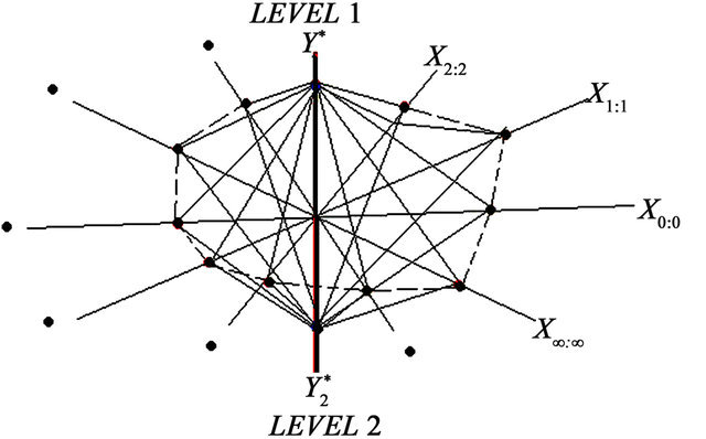
Figure 6. The diamond coordinate space with infinite axes.
offer four axes: Xv1, Xv2, Xv3, Yv. All these four axes are distributed by three independent axes: Xv1, Xv2, Xv3 and one dependent axis: Yv. The Xv1, Xv2, Xv3, Yv axes are fixing positive and negative real numbers R+/−.
In order to plot different values in each axis into the 4-dimensional coordinate space in vertical position, we need to plot each value directly on its axis line. All values were plotted on each axis line need to be joined together by straight lines until we can build pyramidshaped figure with four faces in vertical position is shown in Figure 7.
Additionally, the Yv axis is positioned in the center part of the 4-dimensional coordinate space in vertical position (among the other three axes). It is the convergent point of all the other three axes: Xv1, Xv2, Xv3. In other words, all Xv1, Xv2, Xv3 axes converge always in the Yv axis. The 4-dimensional coordinate system in vertical position is represented by:
([Xv1, Xv2, Xv3], Yv) (5)
5.6. The 4-Dimensional Coordinate Space in Horizontal Position
The 4-dimensional coordinate space in horizontal position offer four axes: Xh1, Xh2, Xh3, Yh. All these four axes are distributed by three independent axes: Xh1, Xh2, Xh3 and one dependent axis: Yh. The Xh1, Xh2, Xh3, Yh are fixing positive and negative real numbers R+/-. In order to plot different values in each axis into the 4-dimensional coordinate space in horizontal position, we need to plot each value directly on its axis line. All values were plotted on each axis line need to be joined together by straight lines until we can build pyramidshaped figure with four faces in horizontal position is shown in Figure 8.
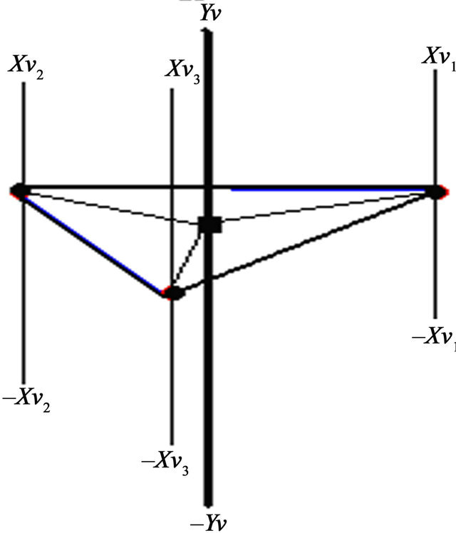
Figure 7. The 4-dimensional coordinate space in vertical position.
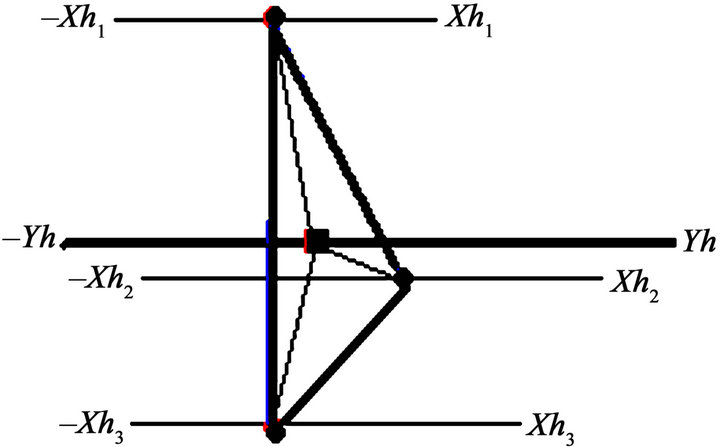
Figure 8. The 4-dimensional coordinate space in horizontal position.
Additionally, the Yh axis is positioned in the center part of the 4-dimensional coordinate space in horizontal position (among the other three axes). It is the convergent point of all the other three axes: Xh1, Xh2, Xh3. In other words, all Xh1, Xh2, Xh3 axes converge always in the Yh axis. The 4-dimensional coordinate system in horizontal position is represented by:
([Xh1, Xh2, Xh3], Yh) (6)
5.7. The 5-Dimensional Coordinate Space in Vertical Position
The 5-dimensional coordinate space in vertical position consists of five vertical axes: Xv1, Xv2, Xv3, Xv4, Yv. All these five axes are distributed by four independent axes: Xv1, Xv2, Xv3, Xv4 and one dependent axis Yv. The Xv1, Xv2, Xv3, Xv4, Yv are fixing positive and negative real numbers R+/-. In order to plot different values in each axis into the 5-dimensional coordinate space in vertical position, we need to plot each value directly on its axis line. All values were plotted on each axis line need to be joined together by straight lines until we can build pyramid-shaped figure with five faces in vertical position is shown in Figure 9. Therefore, the Yv axis is positioned in the center of the 5-dimensional coordinate space in vertical position (among the other four vertical axes). The Yv axis is the convergent axis of all the other four vertical axes: Xv1, Xv2, Xv3, Xv4. The 5-dimensional coordinate system in horizontal position is represented by:
([Xv1, Xv2, Xv3, Xv4], Yv) (7)
5.8. The 5-Dimensional Coordinate Space in Horizontal Position
The 5-dimensional coordinate space in horizontal position consists of five vertical axes: Xh1, Xh2, Xh3, Xh4, Yh. All these five axes are distributed by four independent axes: Xh1, Xh2, Xh3, Xh4 and one dependent axis Yh. The Xh1, Xh2, Xh3, Xh4, Yh are fixing positive and negative real numbers R+/−.
In order to plot different values in each axis into the 5-dimensional coordinate space in horizontal position, we need to plot each value directly on its axis line. All values were plotted on each axis line need to be joined together by straight lines until we can build pyramidshaped figure with five faces in horizontal position is shown in Figure 10.
Therefore, the Yh axis is positioned in the center of the 5-dimensional coordinate space in horizontal position (among the other four horizontal axes). The Yh axis is the convergent axis of all the other four vertical axes: Xh1, Xh2, Xh3, Xh4. The 5-dimensional coordinate system in horizontal position is represented by:
([Xh1, Xh2, Xh3, Xh4], Yh) (8)
5.9. The Infinity Dimensional Coordinates Space under the General Approach
The infinity dimensional coordinates space under the general approach shows a series of n-number of sub-cylinders “C” located in the same general cylinder, each subcylinder in the same general cylinder is fixed by its Level “L” respectively. Where L = {1, 2, 3,...,k}, k → ∞… To plot into the different sub-cylinders in the same general cylinder, it is based on the sub-cylinder location, axis position and ratio. Where XC:L is the independent variable in sub-cylinder “C” at level “L” lying in position
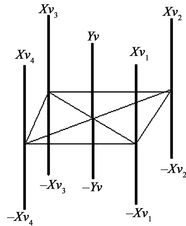
Figure 9. The 5-dimensional coordinate space in vertical position.
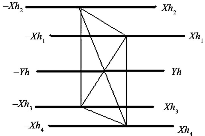
Figure 10. The 5-dimensional coordinate space in horizontal position.
PC:L with value RC:L. The position is based on PC:L by 0◦ ≤ PC:L ≤ 360◦, is the position of XC:L in cylinder “C” at level “L”. And finally the ratios location under the RC:L is the radius corresponding to the XC:L in cylinder “C” at level “L”. Finally, the YC:L is the dependent variable at level “L”. The values of the independent axes XC:L affecting YC:L simultaneously. The infinity dimensional coordinates space under the general approach, its function is given below by:
YC:L = ƒ(XC:L, PC:L, RC:L) (9)
For example, the value of a specific independent axis at time point 1, say X1:1:1 is plotted as R1:1:1 the radius pictured lying on a flat surface at angle P1:1:1 is measured from 0˚ line used for its reference line. The points from the end of the radii are joined to meet in a single point on the top of each sub-cylinder at height Y1:1, the level “L”. The diameter of the sub-cylinder is twice the maximum radius. In order to plot different values in each axis into the infinity dimensional coordinates space under the general approach, we need to plot each value directly on its axis line. All values were plotted on each axis line need to be joined together by straight lines until we can build cone-shaped figure in vertical position is shown in Figure 11.
5.10. The Infinity Dimensional Coordinates Space under the Specific Approach
Basically, the infinity dimensional coordinates space under the specific approach offer a new coordinate system is shown in Expression 10. The basic coordinate space system is formed by three levels of analysis: general-space (i); sub-space (j); micro-space (k). In the case of plotting into this coordinate space start with define our specific general-space (i), sub-space (j), micro-space (k), alphaspace (α) and beta-space (β) respectively.
(α
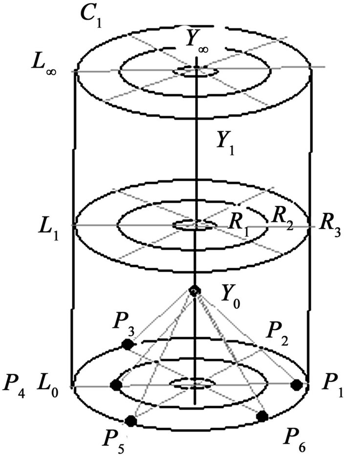
Figure 11. The infinity dimensional coordinates space (general approach).
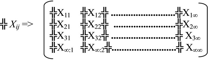
The infinity dimensional coordinates space under the specific approach is available to show different dimensional that is not possible to be observed in the classic 2- dimensional Cartesian coordinate plane and 3-dimensional coordinate space. Hence, the 2-dimensional Cartesian coordinate plane and 3-dimensional coordinate space can be considered as sub-axes systems into the infinity dimensional coordinates space under specific approach. The structure of the infinity dimensional coordinates space under specific approach is formed by infinite general-spaces (i), sub-spaces (j) and micro-spaces (k). There are distributed into different places along the general cylinder is shown in Figure 12. Therefore, the infinity coordinate space under the specific approach starts from the general space zero (i0) until the general space infinity (i∞). And each sub-space starts from sub-space zero (j0) until the sub-space infinity (j∞). Finally, the micro-space starts from micro-space zero (K0) until the micro-space infinity (K∞) is shown in Expression 11.
The infinity dimensional coordinates space under the specific approach is available to connect a large number of micro-spaces (k) distributed into the same sub-space (j) and general space (i) by the application of the interlinkage connectivity of micro-spaces (╦). At the same time, the infinity dimensional coordinates space under the specific approach is also available to connect a large number of general spaces in the same coordinate space. It is based on the application of the inter-linkage connectivity of general-spaces (╬).
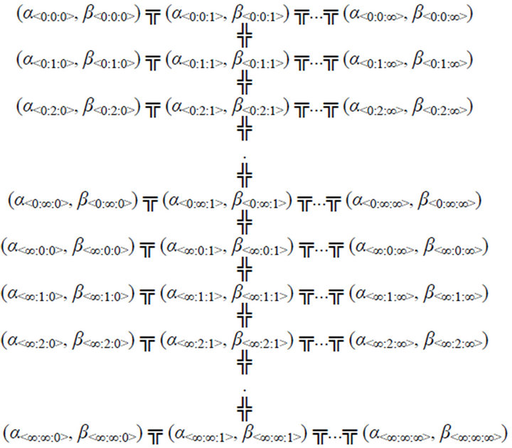 (11)
(11)
5.11. The Inter-Linkage Coordinate Space
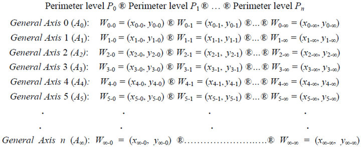
The inter-linkage coordinate space is formed by infinite number of general axes (A0, A1, …, An …), perimeter levels (L0, L1, …, Ln …) and windows refraction (W0,
W1, …, Wn …) are shown in Figure 13. Each window refraction is based on join its sub-x axis (XA-L) with its sub-y axis (YA-L) respectively. Therefore, the window refraction (W0, W1, …, Wn …) is follow by the coordinate Space (XA-L,YA-L). All windows refraction on the same
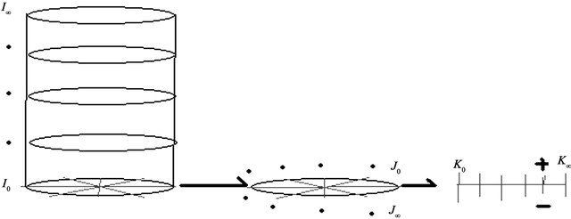
Figure 12. The infinity dimensional coordinates space under the specific approach.
general axis (A0, A1, …, An …) will be joined together under the application of the inter-linkage connectivity of windows refraction represented by “®”. The inter-linkage connectivity of windows refraction is represented by the symbol “®”. The inter-linkage connectivity of windows refraction “®” will inter-connect all windows refraction (W0, W1, …, Wn …) on the same general axis (A0, A1, …, An …) but in different perimeter levels (L0, L1 ,…, Ln …). Moreover, the inter-linkage coordinate system is shown in Expression 12:
 (12)
(12)
Finally, the inter-linkage coordinate space is available to fix a large number of different functions located in different windows refraction (W0, W1 ,…, Wn …), perimeter levels (L1, L2 ,…, Ln …) and general axes (A1, A2, …, An …) are shown in Expression 13:
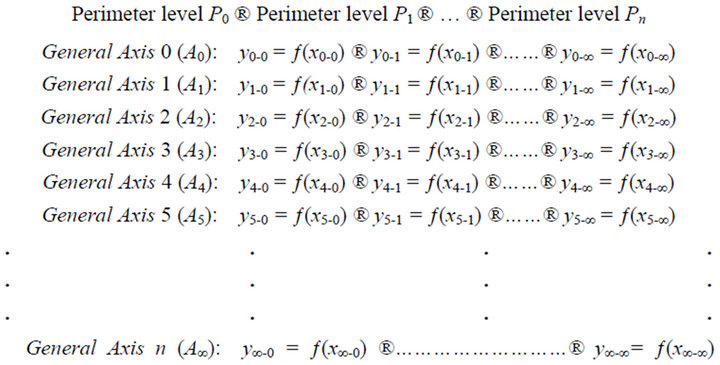 (13)
(13)
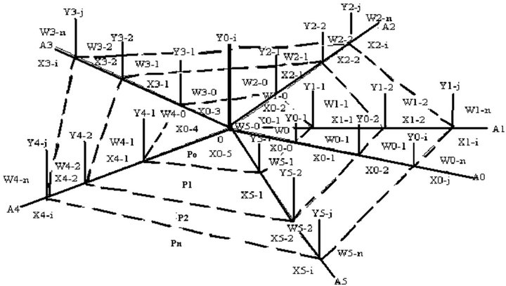
Figure 13. The inter-linkage coordinate space.
5.12. The Cube-Wrap Coordinate Space
The cube-wrap coordinate space is willing to offer an alternative coordinate space. The main objective of the cube-wrap coordinate space is to show unknown dimensions that cannot be visualized by the 2-dimensional Cartesian plane and 3-dimensional coordinate space.
Initially, the cube-wrap coordinate space is divided by two quadrants. The first quadrant is located on the top of the cube-wrap coordinate space that represents all |Xi|- axes. The second quadrant is located under the button of the cube-wrap coordinate space that represents all |Yj|- axes are shown in Figure 14.
In the process to plot on this coordinate space start by plot each value on its axis line respectively. The space that exists between |Xi|-axes and |Yj|-axes will be called “quadratic-space refraction” because each |Xi|-axis has its |Yj|-axis respectively. The construction of the quadratic space refraction is based on two basic steps: the first step is to plot each value on the |Xi|-axis line and |Yj|-axis line, we suggest applying the inter-linkage connectivity of micro-spaces (╦) are shown in Expression 14. Second step is to join the values located on |Xi|-axis and |Yj|-axis by a single straight vertical line.
(|Xi| ╤|Yj|) (14)
We assume that between Xi–axes and Yj–axes exists a common single straight vertical line that joint both set of axes. This common single straight line is called the zero space. Hence, the cube-wrap coordinate space starts from the quadratic space refraction zero (L0) until the quadratic space refraction infinity (L∞). According to the cube wrap coordinate space requests the application of absolute values |R+/−| because the cube wrap coordinate space works only with positive real numbers R+. The final coordinate system to build the cube-wrap coordinate space is shown in Expression 15.
CW = [(S0) = (|X00| ╤ |Y00|) ╬ (S1) = (|X01| ╤ |Y01|) ╬…╬ (S∞) = (|X∞∞| ╤ |Y∞∞|)] (15)
In the final stage of analysis in the cube-wrap space, it is based on its size. We can have three possible stages that the cube-wrap space can experience anytime:
If all values are growing constantly in |Xi| and |Yj| then the cube-wrap experience an expansion-stage (16)
If all values are decreasing constantly in |Xi| and |Yj|
then the cube-wrap experience a contraction-stage (17)
If all values are keeping constant in |Xi| and |Yj| then the cube-wrap experience a static-stage (18)
5.13. The Mega-Space Coordinate Space
The mega-space coordinate space is formed by infinite number of axes in vertical position. Each vertical axis (Xij) show positive integer numbers on the top and negative integer numbers on the bottom in the same vertical axis. At the same time, all the vertical axes can be located by its row number (i) and column number (j) in the mega-space coordinate space is shown in Expression 19.
The idea to apply the mega-surface coordinate space is to build the mega-surface. The mega-surface can show how a large number of variables behave together in the same graphical space. Initially, the construction of the megasurface start by joins each vertical axis value by straight lines with its neighbor vertical axis: front side; left side; right side; back side is shown in Figure 15. To join all axes are necessary to apply the inter-linkage connectivity condition (╬) on all vertical axes simultaneously.
(19)
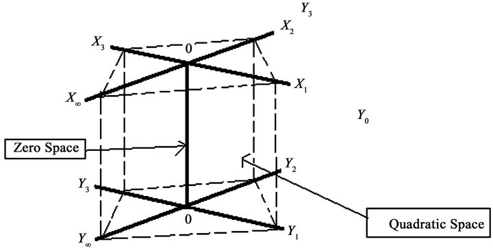
Figure 14. The cube-wrap coordinate space and the cube-wrap space.
The final analysis of the mega-surface is based on its location into the mega-space coordinate space. The possible stages that the mega-surface can experience:
If all Xij values > 0 then the mega-surface shows a expansion stage (20)
If all Xij values = 0 then the mega-surface shows a stagnation stage (21)
If Xij values < 0 then the mega-surface shows a contraction stage (22)
If some Xij is sharing positive, negative or zero values in different vertical axes then the mega-surface shows an unstable performance stage. (23)
5.14. The Cubes Coordinate Space
The cubes coordinate space is formed by infinity number of general axes (A0, A1,…, An). Where each axis shows different levels (L0, L1,…, Ln), perimeters (P0, P1, P2…Pn), and Cubes with different sizes and colors (C0/β, C1/β… Cn/β). Therefore, the coordinate system of the cubes-coordinate space is represented by SA:L:P:C = (Ai, Lj, Pk, Cs/β) respectively. Where i, j, k and s represents different values between 0 and ∞…. And β represent the different colors of each cube in different levels (L0, L1,…, Ln). All the cubes with different sizes and colors in the same axis under the same level (L0, L1 ,…, Ln) and different perimeters (P0, P1, P2…Pn) will be joined together, it is based on the application of the concept is called “macroeconomics links structures” represented by the symbol “@”. Moreover, the cubes-coordinate space coordinate system is shown in Expression 24 and Figure 16.
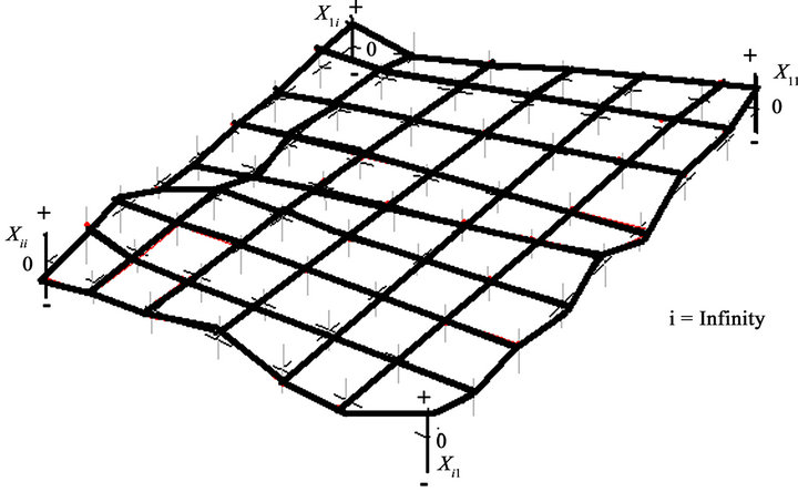
Figure 15. The mega-space coordinate space and the mega-surface.
Figure 16. The cubes-coordinate coordinate space.
 (24)
(24)
Finally, the cubes-coordinate space shows a general function, where the dependent variable is identify by the national economy base “Ne”. The Ne is the final result from ten macroeconomic structures. It is based on link of all macroeconomics structures (S0, S1,…, Sn) under different axes (A1, A2 ,…, An), levels (L1, L2 ,…, Ln), perimeters (P0, P1, P2…Pn) and Cubes with different sizes and colors (C0/β, C1/β… Cn/β) in the same sub-coordinate space respectively, it is shown in Expression 25:
/ΔNe/ = [/ΔAo/ @ /ΔA1 / @ …@ /ΔAn/] (25)
6. Introduction to Econographication
The Econographication is originated by the necessity to generate an alternative and specialized multidimensional graphical modeling for economics, business and finance. In fact, the Econographication main objective is focused on the research, develop and application of multidimensional coordinate spaces to generate different types of multidimensional graphs. Therefore, Econographication will maximize the uses of multi-dimensional graphs to minimize difficulties in the process of meta-database storage and multi-variable data behavior visualization. Hence, the Econographication is defined “as a multi-dimensional graphical modeling theoretical framework can be applied on economics, as well as finance and business.”
Additionally, the Econographication is divided into three large research areas are multidimensional graphs design, multidimensional graphs application and multidimensional graphs simulations. The multidimensional graphs design research area can be 2-dimensional, 3- dimensional and multi-dimensional coordinate spaces under linear and non-linear graph systems, the same section is divided into four sub-sections are coordinate spaces, graphs, charts and diagrams design. The multidimensional graphs application research area are used by two types of data, there are real and experimental data under micro and macro-level analysis in the short and long run is shown in Diagram 1.
The last section is the multidimensional graphs simulations research area, it is divided in two sections are electronic and prototypes. In the case of the electronic area is based on the application and uses of software and solutions. The idea to include prototypes in the multidimensional graphs simulations is to facilitate the easy understanding in the teachinglearning-research process of multi-variable data visualization.
7. Concluding Remarks
Firstly, this research concludes that the 2-dimensional space shows certain limitations to visualize complex economic phenomena simultaneously in the same graphical space and time. Therefore, the multi-dimensional coordinate spaces are available to expand a multidimensional optical effect to visualize different complex economic phenomena in the same graphical space and time according to this research.
Secondly, the Econographication attempts to be an alternative graphical method focus to support the metadatabase
Diagram 1. Econographication research areas.
storage and visualization of multi-variables data behavior, as well as finance and business. The main idea to build Econographication is to offer a new multi-dimensional graphs based on the application of alternative multi-dimensional coordinate spaces can facilitate the study of any economic, finance and business phenomena under macro-level and micro-level of analysis in the short and long run. In summation, the Econographication also will play important role in the research and teaching-learning process of economics through a series of new graphs methods and techniques that can be used by academics, researchers, economist and policy makers.
REFERENCES
- J. Beniger and D. Robyn, “Quantitative Graphics in Statistics: A Brief History,” The American Statistician, Vol. 32, No. 1, 1978, pp. 1-11.
- W. Playfair, “Commercial and Political Atlas and Statistical Breviary (Original Version Was Published in 1786),” Cambridge University Press, Cambridge, 2005.
- F. Edgeworth, “New Methods of Measuring Variation in General Prices,” Journals of the Royal Statistical Society, Vol. 51, 1888, pp. 346-368.
- W. Jevons, “On the Study of Periodic Commercial Fluctuations,” Report of BAAS, Cambridge, 1862.
- H. Maas, “William Stanley Jevons and the Making of Modern Economics,” Cambridge University Press, Cambridge, 2005.
- L. Lafleur, “Discourse on Method, Optics, Geometry, and Meteorology (Translation French to English from Rene Descartes-1637-),” The Liberal Arts Press, New York, 1960.
- A. Cournot, “Mémoire sur les Applications du Calcul des Chances à la Statistique Judiciaire,” Journal des Mathé- matiques Pures et Appliquées, Vol. 12, No. 3, 1838, pp. 257-334.
- P. D. McClelland, “Causal Explanation and Model Building in History, Economics, and the New Economic History,” Cornell University Press, New York, 1975.
- G. Avondo-Bodino, “Economic Applications of the Theory of Graphs,” Gordon & Breach Publishing Group, Newark, 1963.
- J. Hicks, “The Foundations of Welfare Economics,” Economic Journal, Vol. 49, No. 196, 1939, pp. 696-712. doi:10.2307/2225023
- A. Hansen, “Full Recovery or Stagnation?” W. W. Norton & Co., Inc., New York, 1938.
- P. Samuelson, “Foundations of Economic Analysis. US,” Harvard University Press, Cambridge, 1947.
- L. Klein, “The Efficiency of Estimation in Econometric Models,” Cowles Foundation, Yale University, Cowles Foundation Discussion Papers, No. 11, New Haven, 1956.
- A. W. Phillips, “The Relation between Unemployment and the Rate of Change of Money Wage Rates in the United Kingdom, 1861-1957,” Economica, Vol. 25, No. 100, 1958, pp. 283-299.
- A. Okun, “Equality and Efficiency: The Big Tradeoff,” Journal of Economic Literature, Vol. 13, No. 3, pp. 917- 918.
- R. Solow, “A Contribution to the Theory of Economic Growth,” Quarterly Journal of Economics,” Vol. 70, No. 1, 1956, pp. 65-94. doi:10.2307/1884513
- J. Nash, “The Bargaining Problem,” Econometrica, Vol. 18, No. 2, 1950, pp. 155-162. doi:10.2307/1907266
- J. Timbergen, “An Econometrics Approach to Business Cycle Problems, Impasses Economiques,” Herman & C. Publisher, Paris, 1937.
- M. Friedman, “A Monetary and Fiscal Framework for Economic Stability,” American Economic Review, Vol. 38, No. 3, 1948, pp. 245-264.
- R. Barro, “Rational Expectations and the Role of Monetary Policy,” Journal of Monetary Economy, Vol. 2, No. 1, 1976, pp. 1-32. doi:10.1016/0304-3932(76)90002-7
- H. Poincarė, “The Foundations of Sciences: Sciences and Hypothesis, the Value of Sciences, Sciences and Method,” The Sciences Press, New York, 1913.
- J. Brouwer,“Über den Natürlichen Dimensionsbegriff,” Journal für die Reine und Angewandte Mathematik, Vol. 1913, No. 142, 1913, pp. 146-152.
- V. V. Fedorchuk, M. Levin and S. V. Shchepin, “On Brouwer’s Definition of Dimension,” Russian Mathematic Survey, Vol. 54, No. 2, 1999, pp. 432-433. doi:10.1070/RM1999v054n02ABEH000137
- E. V. Shchepin, “Topology of Limit Spaces with Uncountable Inverse Spectra,” Russian Mathematical Surveys, Vol. 31, No. 5, pp. 191-226.
- A. Inselberg and B. Dimsdale, “Multidimensional Lines I: Representation,” SIAM Journal on Applied Mathematics, Vol. 54, No. 2, 1994, pp. 559-577. doi:10.1137/S0036139991216891
- A. Einstein, “Relativity: The Special and the General Theory,” Three Rivers Press, New York, 1952.
- JSTOR: Journal of Economics Section. http://www.elsevier.com
- A. Marshall, “Principles of Economics,” Macmillan and Co., Ltd., London, 1890.
- E. Schlicht, “Isolation and Aggregation in Economics,” Springer-Verlag Publisher, Berlin, 1985. doi:10.1007/978-3-642-70298-3
- M. A. Ruiz Estrada, “Policy Modeling: Definition, Classification, and Evaluation,” Journal of Policy Modeling, Vol. 33, No. 4, 2011, pp. 523-536. doi:10.1016/j.jpolmod.2011.02.003
- M. A. R. Estrada, “Econographicology,” International Journal of Economic Research, Vol. 4, No. 1, 2007, pp. 75- 86.
- M. A. R. Estrada, “Mulidimensional Coordinate Spaces,” International Journal of Physical Sciences, Vol. 6, No. 3, 2011, pp. 340-357.
NOTES
1American Economic Review; Canadian Journal of Economics; Econometrica; Economica; Economic History Review; Economic Journal; International Economic Review; Journal of Economic History; Journal of Economic Literature; Journal of Political Economy; Oxford Economic Papers; Quarterly Journal of Economics; Review of Economic Studies; Review of Economics and Statistics; Canadian Journal of Economics and Political Science; Journal of Economic Abstracts; Contributions to Canadian Economics; Journal of Labor Economics; Journal of Applied Econometrics; Journal of Economic Perspectives; Publications of the American Economic Association; Brookings Papers on Economic Activity. Microeconomics and American Economic Association Quarterly (JSTOR, [14]).