Journal of Environmental Protection
Vol.4 No.12A(2013), Article ID:40509,10 pages DOI:10.4236/jep.2013.412A1001
Feed-Forward Artificial Neural Network Model for Air Pollutant Index Prediction in the Southern Region of Peninsular Malaysia
![]()
1East Coast Environmental Research Institute (ESERI), Universiti Sultan Zainal Abidin, Gong Badak Campus, Kuala Terengganu, Malaysia; 2School of Environmental and Natural Resource Sciences, Faculty of Science and Technology, Universiti Kebangsaan Malaysia, Bangi, Malaysia; 3Department of Chemistry, Faculty of Science, Universiti Malaya, Kuala Lumpur, Malaysia; 4Kulliyyah of Science, International Islamic University Malaysia, Kuantan, Malaysia.
Email: *hafizanj@gmail.com
Copyright © 2013 Azman Azid et al. This is an open access article distributed under the Creative Commons Attribution License, which permits unrestricted use, distribution, and reproduction in any medium, provided the original work is properly cited. In accordance of the Creative Commons Attribution License all Copyrights © 2013 are reserved for SCIRP and the owner of the intellectual property Azman Azid et al. All Copyright © 2013 are guarded by law and by SCIRP as a guardian.
Received September 6th, 2013; revised October 8th, 2013; accepted November 5th, 2013
Keywords: Air Pollutant Index (API); Principal Component Analysis (PCA); Artificial Neural Network (ANN); Rotated Principal Component Scores (RPCs); Feed-Forward ANN
ABSTRACT
This paper describes the application of principal component analysis (PCA) and artificial neural network (ANN) to predict the air pollutant index (API) within the seven selected Malaysian air monitoring stations in the southern region of Peninsular Malaysia based on seven years database (2005-2011). Feed-forward ANN was used as a prediction method. The feed-forward ANN analysis demonstrated that the rotated principal component scores (RPCs) were the best input parameters to predict API. From the 4 RPCs, only 10 (CO, O3, PM10, NO2, CH4, NmHC, THC, wind direction, humidity and ambient temp) out of 12 prediction variables were the most significant parameters to predict API. The results proved that the ANN method can be applied successfully as tools for decision making and problem solving for better atmospheric management.
1. Introduction
Nowadays, air pollution becomes a major environmental issue throughout the world. Sudden occurrences of high concentration of vehicular and industrial exhaust emissions are the episodes of air pollution in the urban areas [1]. With the rapid economic growth, air pollution is the main subject that has been adversely affecting human health, agricultural crops, animals and ecosystems. It can unavoidably cause damages to buildings, monuments and statues. Moreover, not only it reduces visibility; it even interferes with aviation.
The rapid industrial development and urbanization in the southern region of Peninsular Malaysia have contributed to high levels of atmospheric pollutants to the environment. The problems of severe air quality exist in highly urbanized areas [2]. Mobiles, stationary and transboundary sources are the major sources of air pollution in Malaysia [3,4]. Mobile sources include motor vehicle, are the main sources of air pollutants in Malaysia [4,5]. The stationary sources within the study area are coming from the emissions of urban construction works, quarries, petrochemical and power plants [6]. The uncontrolled wildfires, earthquake and volcanic eruption from neighbouring countries are the examples of trans-boundary sources within the study area [4,7].
Symptoms such as eye and skin irritation, nose, throat, headache, fatigue, dizziness, and difficulty in breathing are general of health effect experienced by human due to poor air quality [8]. Worldwide, there are more deaths from indigent air quality than from automobile accident [9]. The particulate matter under 10 microns (PM10) and ground-level ozone (O3) are the most pollutants that influence human health [10,11].
Air pollutant index (API) has been used as an indicator of air quality in Malaysia since 1989 [4,12]. Five criteria of air pollutants—ground level-ozone (O3), carbon monoxide (CO), nitrogen dioxide (NO2), sulphur dioxide (SO2), and particulate matter under 10 microns (PM10) were used as API calculation. The highest value of the individual sub-index is taken as the API value [5,12]. The API values are used to advise or caution the public in lieu of health effects [13].
The air-quality prediction is important for planning, proper actions and controlling strategies. Due to the concern, artificial neural network (ANN) has been applied for prediction purposes, especially on air quality [14,15]. The ANN can be used to evaluate the predictive performance [16-20], and gives a better performance comparable to other models [21]. Unlike other techniques, ANN is capable in the recognition of non-linear patterns between the variables and complex patterns in data sets, which are not well described by simple mathematical formulae [22]. The ANN can be trained accurately when presented with a new data set [23-25].
This study aims to classify variables’ predictor by using the PCA method. This study also aims to predict API in the Southern Region of Peninsular Malaysia uses the varimax factors data, generated by the PCA method as input variables in ANN models.
2. Materials and Methods
2.1. Study Area
In this study, seven air monitoring stations were selected due to located within the area of industries and high population density, and known as the most developed area in Malaysia. Figure 1 and Table 1 illustrate the air-quality monitoring area and the description of sampling stations. The stations were identified based on the availability of data for the seven years of the period (2005-2011). The daily traffic density is classified as moderate to high and the peak periods found during morning and evening. There is no major natural disaster (such as typhoon, volcanic eruption) was occurring in these areas, which make the air-quality monitoring in the southern region of Peninsular Malaysia is under control.

Figure 1. Location of continuous air quality monitoring stations in the Southern Region of Peninsular Malaysia.
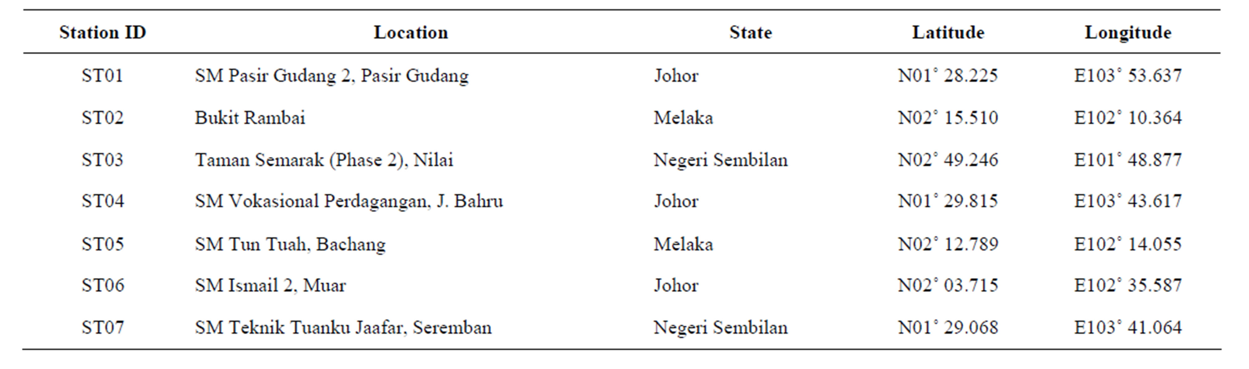
Table 1. Detail description of air quality monitoring stations of the study area.
2.2. Data Pre-Treatment
In this study, the prediction model was developed using 232,505 datasets (13 parameters × 17,885 observations). The recorded data were provided by the Air Quality Division, Department of Environment Malaysia. The air quality and meteorological parameters used in this study are carbon monoxide (CO), nitrogen dioxide (NO2), methane (CH4), ozone (O3), sulphur dioxide (SO2), nonmethane hydrocarbon (NmHC), total hydrocarbon (THC), particulate matter under 10 microns (PM10), wind direction, wind speed, ambient temperature and humidity.
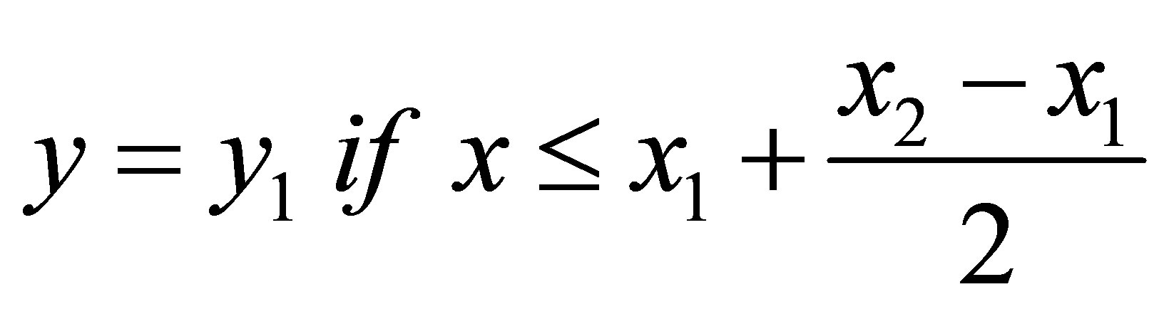
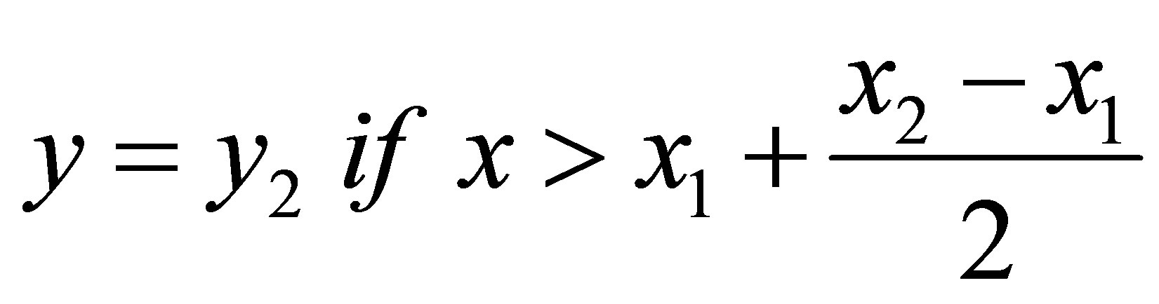
Less than 3% of missing data were found from the overall data and then the nearest neighbour method was applied for estimation of missing values [26] based on the endpoints of the gaps using Equation (1):
or
 (1)
(1)
where y is the interpolant, x is the time point of the interpolant, y1 and x1 are the coordinates of the starting point of the gap, and y2 and x2 are the endpoints of the gap.
2.3. Principal Component Analysis (PCA)
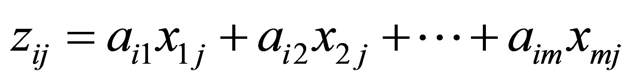
In this study, PCA was performed to generate the principal components (PCs) and used as input variables in the API prediction model using ANN approach. The PCs can expressed as Equation (2):
 (2)
(2)
where z is the component score, a is the component loading, x is the measured value of the variable, i is the component number, j is the sample number, and m is the total number of variables.
The PCs generated by the PCA is advisable to rotate using varimax rotation due to not readily interpreted [4,12]. Only the PCs with eigenvalues more than 1 are considered significant in the varimax rotations analysis [27] in order to obtain new groups of variable (varimax factors, VFs). The number of VFs from varimax rotations is equal to the number of variable in accordance with common features and can include unobservable, hypothetical, and latent variables [28]. The VF coefficient with absolute values greater than 0.75 is selected due to having significant factor loadings [29]. The analysis of PCA was implemented using XLSTAT 2013 add-in software.
2.4. Artificial Neural Network (ANN)—API Prediction Model
Artificial Neural Network (ANN) is an information processing unit analog to the neuron network in biological system [30]. ANN has the ability to learn complex patterns of information and generalize it for the prediction, classification and clustering activities [31]. ANN is widely known as the method to provide better predicting, which the results are depending on the use of a large number of inputs [32]. ANN also can be used to learn future predicting events based on the patterns that have been observed in the historical data, to classify unseen data into pre-defined groups which it based on the observed characteristics, and it was able to cluster the data into natural groups based on the similarity of characteristics in data [31].
In this study, feed-forward ANN (supervised models) was used for prediction purposes and to determine the most significant parameters affecting API values. This technique only forwards information transfer but no feedback information [33]. This model consists of three layers, known as the input layer, hidden layer and output layer. The total numbers of input (independent test set) and hidden layer were determined by the nature of the problem to the research and has been varied depending on predicting horizon, whereas the output layer (dependent test set) has a single node [34]. A total of 17,885 data sets were used in this analysis. For developing the ANN model, the data were divided into three sets: 60% of the data for the whole training set (10,731 data), follows with 20% of the whole data for testing, and validation set (3577 data) respectively [8].
Three different feed-forward ANN models were developed with different input variables—Model A (this model was developed based on the original raw data, twelve parameters), Model B (this model was developed based on the twelve PCs without varimax rotation) and Model C (this model was developed using factor scores of rotated (varimax rotation) PCs with eigenvalues greater than 1 as input variables). For the Model C, prediction of the API was performed using two to four rotated principal components (RPCs), separately. The network structure for the feed-forward ANN model was presented in Figure 2.
Trial-and-error procedure between one to twelve hidden layers in the network structure was examined in order to approximate any nonlinear function with any level of accuracy and it was used to search the best model for prediction of API values. Based on theoretical studies, a network with a small number of nodes shall probably fail to learn the data, while too many nodes shall fatefully over fit the training patterns in the network and give a poor generalization performance’s result, especially when dealing with noisy data in predicting problems [32].
There are two different criteria that have been used to evaluate the effectiveness of each network and its ability to make precise prediction [35], namely correlation of determination (R2) and root mean square error (RMSE). The R2 efficiency criterion is expressed as Equation (3):
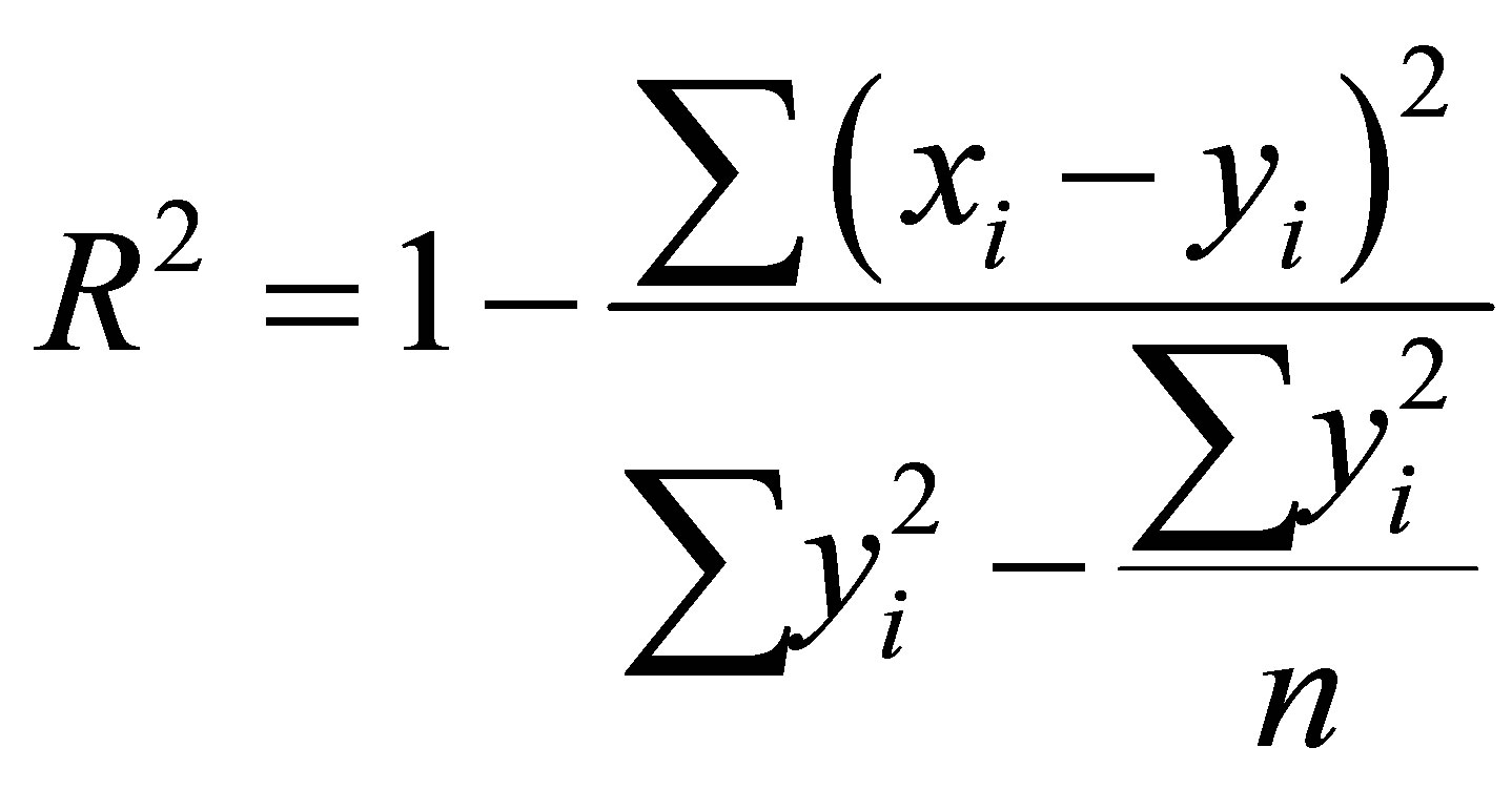 (3)
(3)
While, the RMSE is calculated using Equation (4):
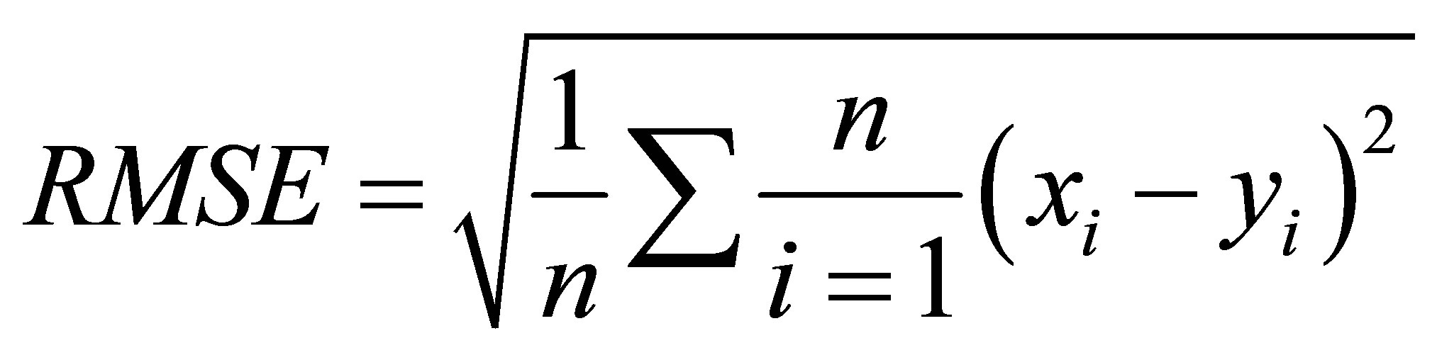 (4)
(4)
where xi denotes the observed data, yi is the predicted data and n is the number of observations and representing the percentage of the initial uncertainty which explained by the model.
Here, the lower of RMSE (RMSE = 0) and the highest of R2 (R2 = 1), the more accurate the prediction is [34]. Then, the predicted values of ANN models were compared each other to obtain parsimonious model (a model that depends on as few variables as necessary) for API prediction. The ANN models were performed using JMP10 software, which this tool offers flexible and easy to apply.
3. Results and Discussion
3.1. Predicting of the API Using Feed-Forward ANN Model
From the PCA result, out of the twelve principal components (PCs) generated, only four PCs with eigenvalues
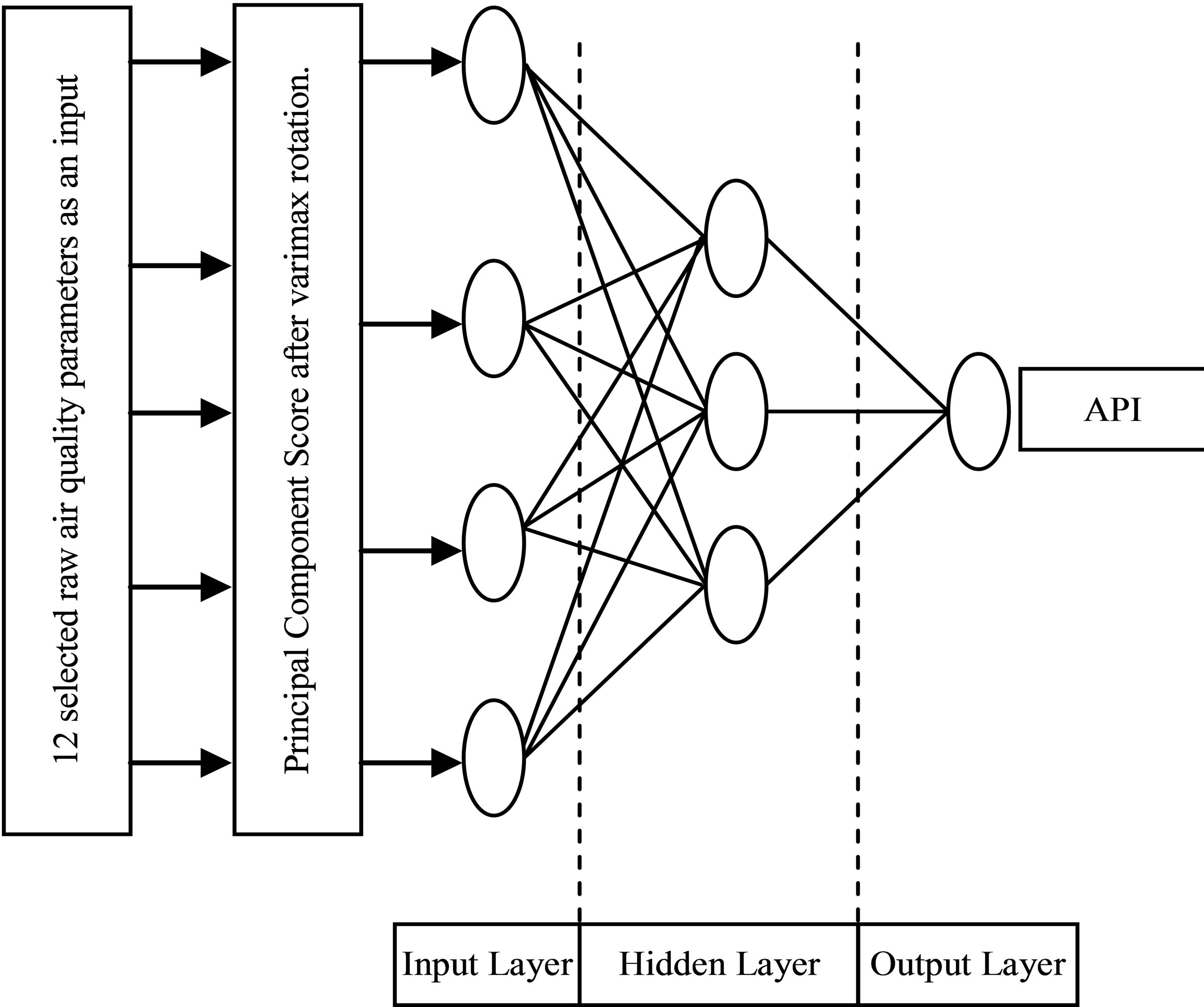
Figure 2. Example of feed-forward ANN model network structure of this study.
greater than 1 was selected for the feed-forward ANN input selection parameters representing 69.8% of the total variance (Table 2). The results of the four rotated PCs (RPCs) from the loading of PCA are given in Table 3. Ten variables with strong loadings (noted in bold) were included in four selected RPCs.
Table 4 and Figure 3 show the prediction performance of feed-forward ANN models for forecasting API using different combinations of PC scores as input variables. In the Model A (original raw parameters as inputs), the optimum neuron in the hidden layers was eight neurons. The R2 values of training, testing and validation are 0.694, 0.695 and 0.724 respectively. The results produced by RMSE for training, testing and validation are 7.915, 7.943 and 7.941 respectively.
In the Model B (twelve principal component scores as inputs), the three layer network was used with twelve neurons in the input layer, eleven neurons in the hidden layer and one neuron in the output layer with 100% variation, which explained the R2 values of training, testing and validation are 0.714, 0.749 and 0.736 respectively. Meanwhile, the RMSE values of training, testing and validation for the Model B are 7.574, 7.151 and 7.562 respectively.
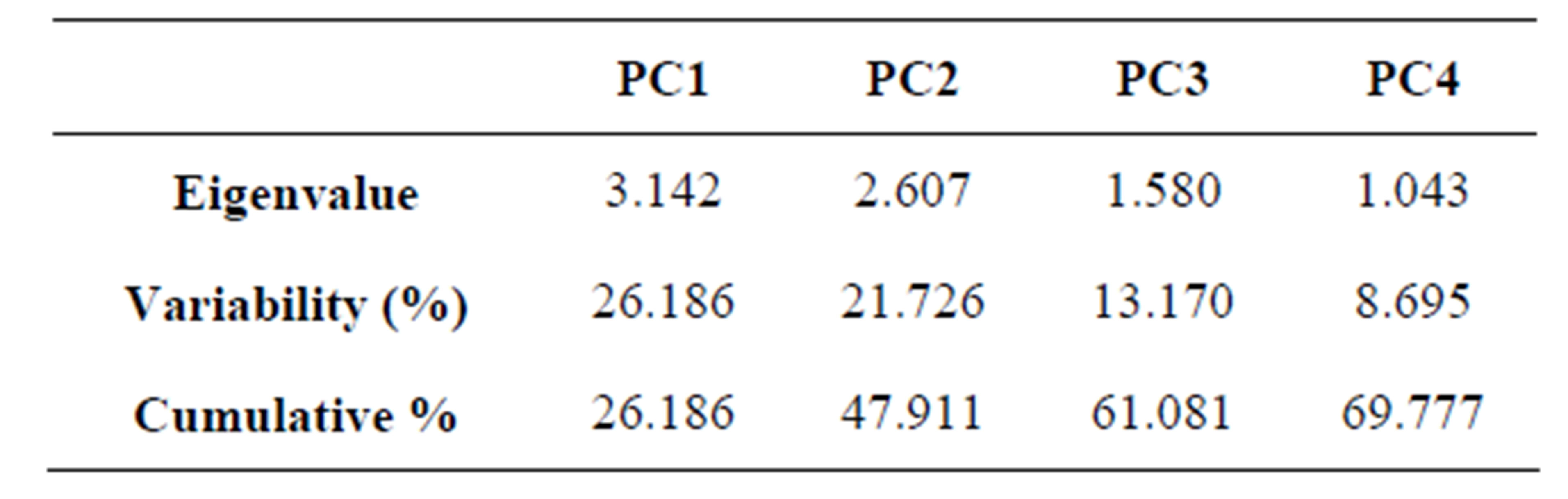
Table 2. Descriptive statistics of selected original PCs.
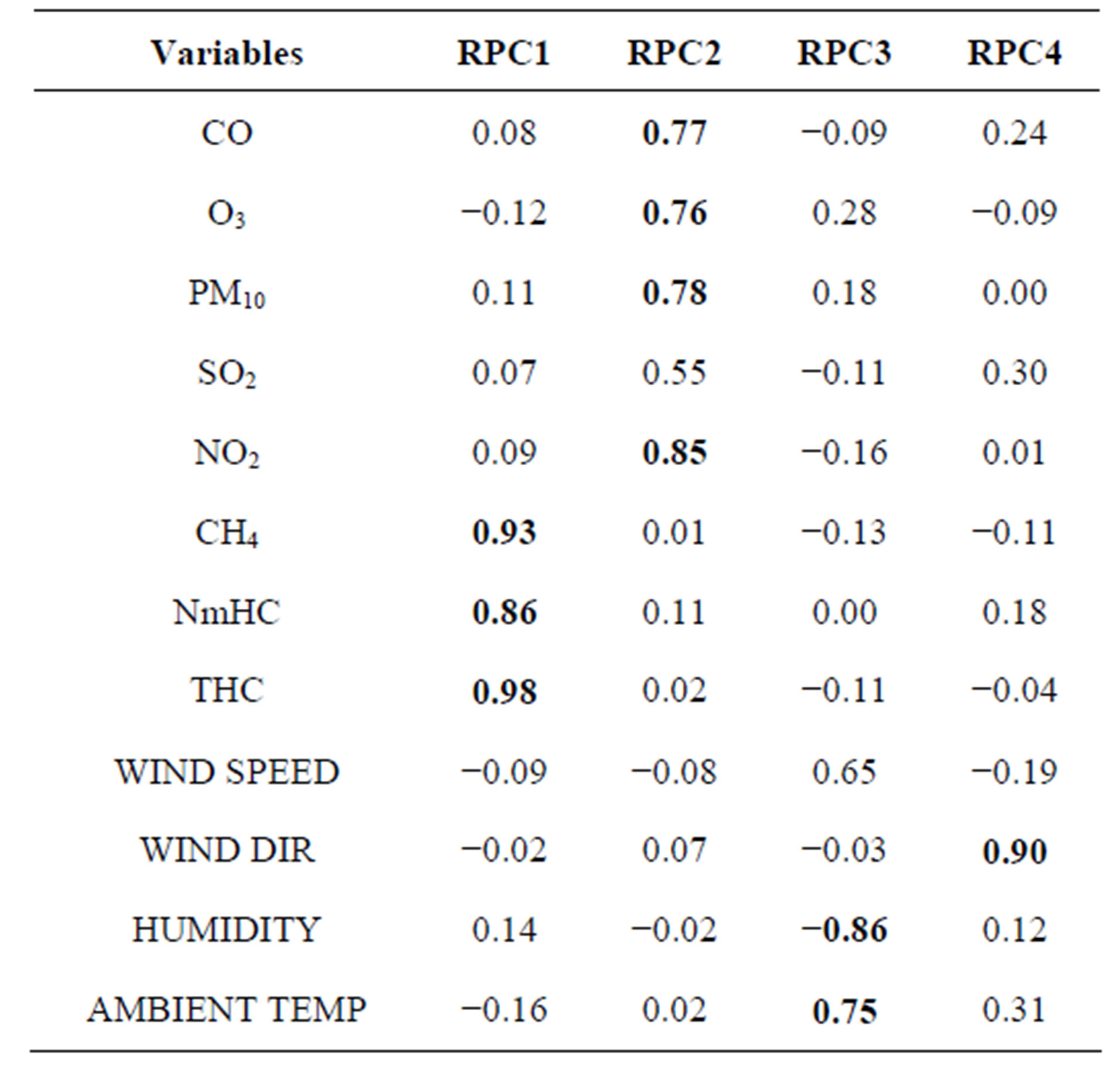
Table 3. Rotated factor loadings using four PCs.
In the Model C, three types of ANN sub-models were developed. For each sub-models, the optimum neuron in the hidden layer was seven neurons. The feed-forward ANN model using the first two RPCs (RPC1 and RPC2) as input neurons indicates it does not perform well for the training, testing and validation phases with the cumulative percentage explaining only 47.9% variation. The R2 values for training, testing and validation are 0.270, 0.347 and 0.360 respectively. Furthermore, the RMSE values of training, testing and validation for the two RPCs are 11.960, 11.637 and 11.553 respectively. The second sub-model of feed-forward ANN in Model B uses three RPCs (RPC1, RPC2 and RPC3) as input parameters. The cumulative percentage of this sub-model showing the variance given by three RPCs is 61.1% with the values of R2 are 0.317, 0.399 and 0.372 in training, testing and validation respectively. The results produced by RMSE are 11.587, 11.119 and 11.896 for training, testing and validation respectively. From the results, the highest accuracy in predicting API is given by the third sub-model of feed-forward ANN, which contains four RPCs (69.8% of variation) with R2 value of 0.357, 0.394 and 0.404 for training, testing and validation respectively. While, the RMSE values of training, testing and validation for the four RPCs are 11.269, 11.163 and 11.494 respectively. Based on the three sub-models, it is clear that the API prediction performance increases with the increase in the total number of input variables.
From the observations, the prediction performance of the feed-forward ANN model using four RPCs has significantly different from the original raw parameters and twelve PCs. However, the feed-forward ANN model from four RPCs is a better input due to use fewer variables (ten parameters) than the Model A and Model B (twelve parameters).
3.2. Comparative Performance of Feed-Forward ANN for Model A, Model B and Model C
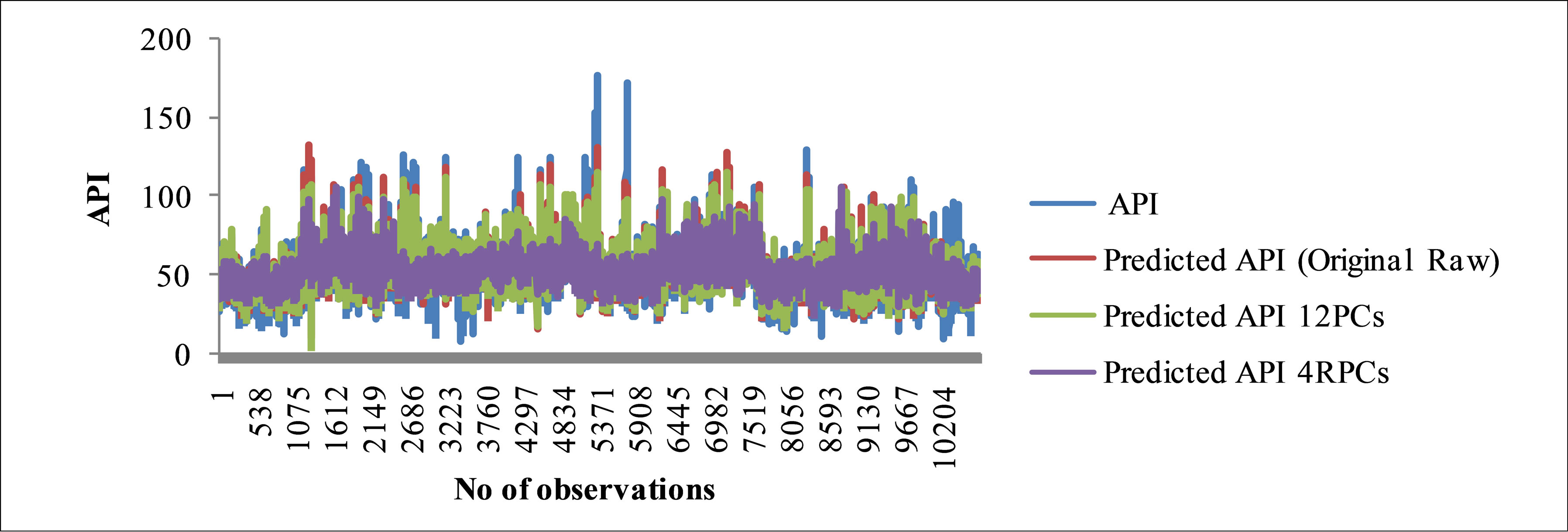
Figures 4(a)-(c) demonstrated the performance of the feed-forward ANN model based on actual API and predicted API using original raw data parameters (Model A), twelve PCs (Model B) and four RPCs (Model C) input selection. The models illustrate how network performance changes over the range of API values. Based on the Figures 4(a)-(c), Model C shows the “best result” compares to Model A and B for training, testing and validation data set due to the majority of predicted data is not significantly different from actual data. Although the R2 values of training, testing and validation set for Model A (0.694, 0.695 and 0.724 respectively) and Model B (0.714, 0.749 and 0.736 respectively) are more accurately than Model C (0.357, 0.394 and 0.404 respectively), but
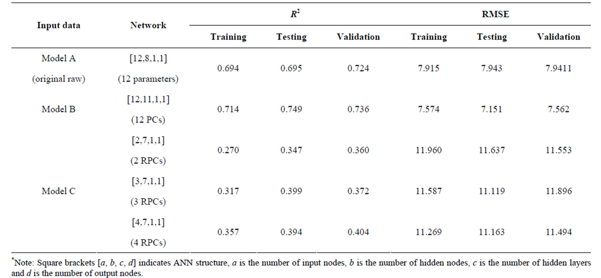
Table 4. The prediction performance of feed-forward ANN models.
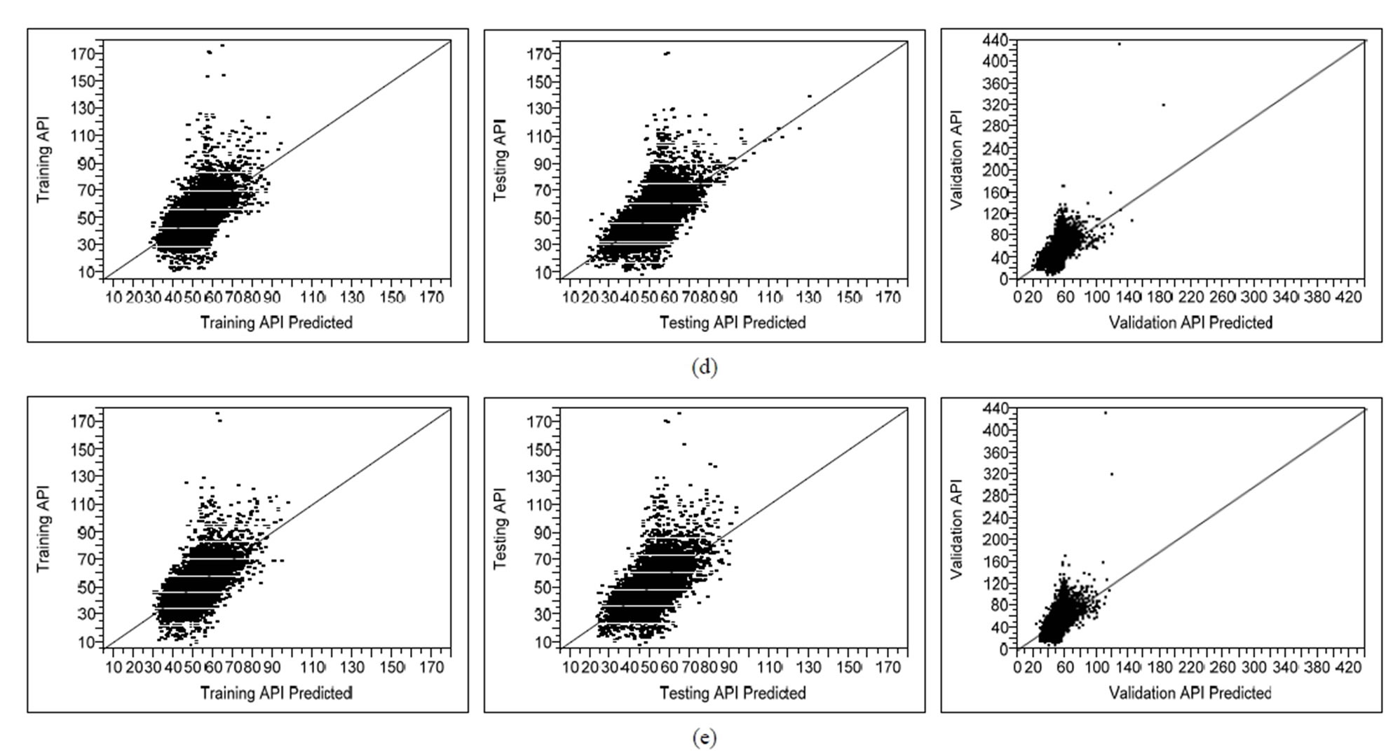
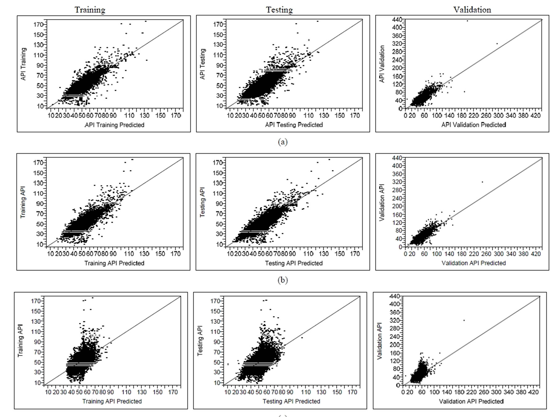
Figure 3. Scatter plot diagram of the prediction performance (actual by predicted plot) for different combination of PC scores during training, testing and validation phases: (a) Original raw data; (b) 12 original PCs; (c) 2 RPCs; (d) 3 RPCs; (e) 4 RPCs.
 (a)
(a)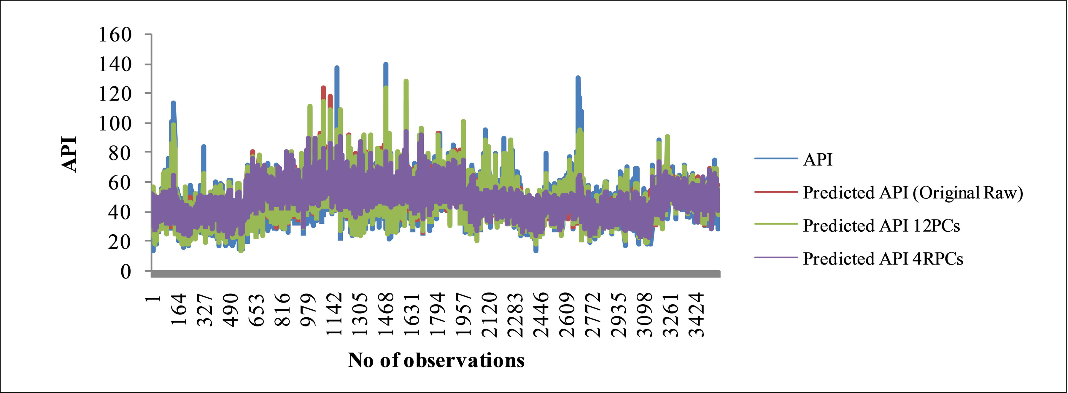 (b)
(b)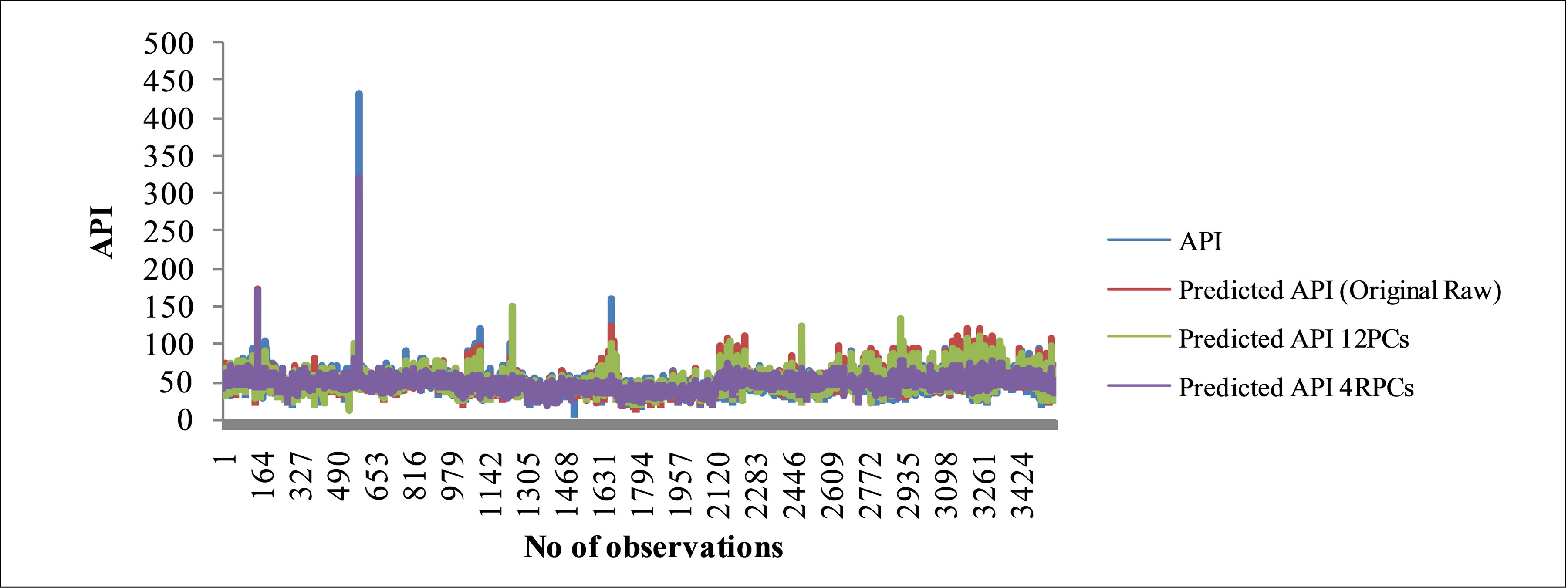 (c)
(c)
Figure 4. Graphs show measured and predicted API for 12 parameters (original raw) feed-forward ANN model, 12 PCs feed-forward ANN model and 4 RPCs feed-forward ANN model for (a) Training; (b) Testing; (c) Validation phase.
the Model C uses fewer variables and is far less complex than Model A which the advantage over this model. Therefore, it proved that the feed-forward ANN architecture is able to predict API values from all available inputs with negligible precision.
4. Conclusions
In this study, a combination of PCA and ANN method was used to predict API based on 12 historical air quality parameters. The original raw data were used as a reference of predictor. Two different approaches were used: un-rotated original PCs (twelve original PCs) and varimax rotated PCs in order to obtain the latent variables as feed-forward ANN inputs.
The findings show that the feed-forward ANN model from twelve original PCs (Model A) as input gives high value of R2. However, the Model B (un-rotated twelve PCs) gives better in prediction compared to the Model A in term of R2 value. Using four PCs, the significant loadings for this study are known as CH4, NmHC, THC, CO, O3, PM10, NO2, humidity, ambient temperature and wind direction. Although, the prediction performance of the Model C (the model based on these 10 PC scores) is lower than Model A and Model B, but the models can predict the API within acceptable accuracy. It means that the use of rotated PC scores based models is more efficient and effective due to reduction of predictor variables without losing important information. It has also proved that these RPCs-ANN models are absolutely very useful tools in helping decision making and problem solving for better atmospheric management of the local environment.
5. Acknowledgements
The authors acknowledge the Air Quality Division of the Department of Environment (DOE) under the Ministry of Natural Resource and Environment, Malaysia for their permission to utilise air quality data for this study. The authors also gratefully acknowledge the Faculty of Environmental Studies, Universiti Putra Malaysia (UPM), School of Environmental and Natural Resource Science, Universiti Kebangsaan Malaysia (UKM) and the Chemistry Department of the Universiti Malaya, who have provided us with secondary data and valuable advice, guidance and support.
REFERENCES
- S. M. S. Nagendra and M. Khare, “Modelling Urban Air Quality Using Artificial Neural Network,” Clean Technologies and Environmental Policy, Vol. 7, No. 2, 2005, pp. 116-126. http://dx.doi.org/10.1007/s10098-004-0267-6
- S. Z. Azmi, M. T. Latif, A. S. Ismail, L. Juneng and A. A. Jemain, “Trend and Status of Air Quality at Three Different Monitoring Stations in the Klang Valley, Malaysia,” Air Quality Atmosphere and Health, Vol. 3, No. 1, 2010, pp. 53-64. http://dx.doi.org/10.1007/s11869-009-0051-1
- R. Afroz, M. N. Hassan and N. A. Ibrahim, “Review of Air Pollution and Health Impacts in Malaysia,” Environmental Research, Vol. 92, No. 2, 2003, pp. 71-77. http://dx.doi.org/10.1016/S0013-9351(02)00059-2
- S. N. S. A. Mutalib, H. Juahir, A. Azid, S. M. Sharif, M. T. Latif, A. Z. Aris, S. M. Zain and D. Dominick, “Spatial and Temporal Air Quality Pattern Recognition Using Environmetric Techniques: A Case Study in Malaysia,” Environmental Science: Processes & Impacts, Vol. 15, No. 9, 2013, pp. 1717-1728. http://dx.doi.org/10.1039/c3em00161j
- M. B. Awang, A. B. Jaafar, A. M. Abdullah, M. B. Ismail, M. N. Hassan, R. Abdullah, S. Johan and H. Noor, “Air Quality in Malaysia: Impacts, Management Issue and Future Challenges,” Respirology, Vol. 5, No. 2, 2000, pp. 183-196. http://dx.doi.org/10.1046/j.1440-1843.2000.00248.x
- B. T. Heninger and F. A. Shah, “Control of Stationary and Mobile Source Air Pollution: Reducing Emissions of Hydrocarbons for Ozone Abatement in Connecticut,” Land Economics, Vol. 74, No. 4, 1998, pp. 497-513. http://dx.doi.org/10.2307/3146881
- H. H. Jamal, M. S. Pillay, H. Zailina, B. S. Shamsul, K. Sinha, Z. Zaman Huri, S. L. Khew, S. Mazrura, S. Ambu, A. Rahimah and M. S. Ruzita, “A Study of Health Impact & Risk Assessment of Urban Air Pollution in Klang Valley,” UKM Pakarunding Sdn Bhd, Kuala Lumpur, 2004, p. 100.
- H. Xie, F. Ma and Q. Bai, “Prediction of Indoor Air Quality Using Artificial Neural Networks,” IEEE Computer Society of 2009 Fifth International Conference on Natural Computation, 2009, pp. 414-418. http://dx.doi.org/10.1109/ICNC.2009.502
- S. Deleawe, J. Kusznir, B. Lamb and D. Cook, “Predicting Air Quality in Smart Environments,” Journal of Ambient Intelligence and Smart Environments, Vol. 2, No. 2, 2010, pp. 145-154.
- M. Ezzati, A. D. Lopez, A. Rodgers, S. Vander Hoorn and C. J. Murray, “Comparative Risk Assessment Collaborating Group: Selected Major Risk Factors and Global and Regional Burden of Disease,” Lancet, Vol. 360, No. 9343, 2002, pp. 1347-1360. http://dx.doi.org/10.1016/S0140-6736(02)11403-6
- W. R. W. Mahiyudin, M. Sahani, R. Aripin, M. T. Latif, T. Q. Thach and C. M. Wong, “Short-Term Effects of Daily Air Pollution on Mortality,” Atmospheric Environment, Vol. 65, 2013, pp. 69-79. http://dx.doi.org/10.1016/j.atmosenv.2012.10.019
- D. Dominick, H. Juahir, M. T. Latif, S. M. Zain and A. Z. Aris, “Spatial Assessment of Air Quality Patterns in Malaysia Using Multivariate Analysis,” Atmospheric Environment, Vol. 60, pp. 172-181. http://dx.doi.org/10.1016/j.atmosenv.2012.06.021
- M. M. Kamal, R. Jailani and R. L. A. Shauri, “Prediction of Ambient Air Quality Based on Neural Network Technique,” 4th Student Conference on Research and Development, Selangor, 27-28 June 2006, pp. 115-119. http://dx.doi.org/10.1109/SCORED.2006.4339321
- S. V. Barai, A. K. Dikshit and S. Sharma, “Neural Network Models for Air Quality Prediction: A Comparative Study,” In: A. Saad, et al. Eds., Soft Computing in Industrial Application, Advance in Soft Computing, SpringerVerlag, Berlin, Vol. 39, 2007, pp. 290-305. http://dx.doi.org/10.1007/978-3-540-70706-6_27
- W. Wang, Z. Xu and J. W. Lu, “Three Improved Neural Network Models for Air Quality Forecasting,” Engineering Computations, Vol. 20, No. 2, 2003, pp. 192-210. http://dx.doi.org/10.1108/02644400310465317
- M. Hubbard and W. G. Cobourn, “Development of a Regression Model to Forecast Ground-Level Ozone Concentration in Louisville, KY,” Atmospheric Environment, Vol. 32, No. 14-15, 1998, pp. 2637-2647. http://dx.doi.org/10.1016/S1352-2310(97)00444-5
- J. M. Davis and P. Speckman, “A Model for Predicting Maximum and 8 h Average Ozone in Houston,” Atmospheric Environment, Vol. 33, No. 16, 1999, pp. 2487- 2500. http://dx.doi.org/10.1016/S1352-2310(98)00320-3
- P. Perez and J. Reyes, “An Integrated Neural Network Model for PM10 Forecasting,” Atmospheric Environment, Vol. 40, 2006, pp. 2845-2851. http://dx.doi.org/10.1016/j.atmosenv.2006.01.010
- U. Brunelli, U. Piazza and L. Pignato, “Two-Day Ahead Prediction of Daily Maximum Concentrations of SO2, O3, PM10, NO2, CO in the Urban Area of Palermo, Italy,” Atmospheric Environment, Vol. 41, No. 14, 2007, pp. 2967-2995. http://dx.doi.org/10.1016/j.atmosenv.2006.12.013
- S. Thomas and R. B. Jacko, “Model for Forecasting Expressway Fine Particulate Matter and Carbon Monoxide Concentration: Application of Regression and Neural Network Model,” Air & Waste Management Association, Vol. 57, No. 4, 2007, pp. 480-488. http://dx.doi.org/10.3155/1047-3289.57.4.480
- K. D. Karatzas and S. Kaltsatos, “Air Pollution Modelling with the Aid of Computational Intelligence Methods in Thessaloniki, Greece,” Simulation Modelling Practice and Theory, Vol. 15, 2007, pp. 1310-1319. http://dx.doi.org/10.1016/j.simpat.2007.09.005
- S. Palani, P. Tkalich, R. Balasubramanian and J. Palanichamy, “ANN Application for Prediction of Atmospheric Nitrogen Deposition to Aquatic Ecosystems,” Marine Pollution Bulletin, Vol. 62, 2011, pp. 1198-1206. http://dx.doi.org/10.1016/j.marpolbul.2011.03.033
- S. H. Sohn, S. C. Oh and Y. K. Yeo, “Prediction of Air Pollutants by Using an Artificial Neural Network,” Korean Journal of Chemical Engineering, Vol. 16, No. 3, 1999, pp. 382-387. http://dx.doi.org/10.1007/BF02707129
- A. Kurt, B. Gulbagai, F. Karaca and O. Alagha, “An Online Air Pollution Forecasting System Using Neural Networks,” Environment International, Vol. 34, No. 5, 2008, pp. 592-598. http://dx.doi.org/10.1016/j.envint.2007.12.020
- A. Mahboubeh, A. Afsaneh and Z. Gholamreza, “The Potential of Artificial Neural Network Technique in Daily and Monthly Ambient Air Temperature Prediction,” International Journal of Environmental Science and Development, Vol. 3, No. 1, 2012, pp. 33-38.
- H. Junninen, H. Niska, K. Tuppurainen, J. Ruuskanen and M. Kolehmainen, “Methods for Imputation of Missing Values in Air Quality Data Set,” Atmospheric Environment, Vol. 38, 2004, pp. 2895-2907. http://dx.doi.org/10.1016/j.atmosenv.2004.02.026
- J.-O. Kim and C. W. Mueller, “Introduction to Factor Analysis: What It Is and How to Do It,” Quantitative Applications in the Social Science Series, Sage University Press, Newbury Park, 1987, p. 80.
- M. Vega, R. Pardo, E. Barrato and L. Deban, “Assessment of Seasonal and Polluting Effects on the Quality of River Water by Exploratory Data Analysis,” Water Research, Vol. 32, 1998, pp. 3581-3592. http://dx.doi.org/10.1016/S0043-1354(98)00138-9
- J. Stevens, “Applied Multivariate Statistics for the Social Science,” Hill Sdale, New Jersey, 1986, p. 515.
- D. Silverman and J. A. Dracup, “Artificial Neural Networks and Long-Range Precipitation in California,” Journal of Applied Meteorology, Vol. 31, No. 1, 2000, pp. 57- 66. http://dx.doi.org/10.1175/1520-0450(2000)039<0057:ANNALR>2.0.CO;2
- H. Hakimpoor, K. A. Arshad, H. H. Tat, N. Khani and M. Rahmandoust, “Artificial Neural Networks’ Application in Management,” World Applied Sciences Journal, Vol. 14, No. 7, 2011, pp. 1008-1019.
- A. Chaloulakou, G. Grivas and N. Spyrellis, “Neural Network and Multiple Regression Model for PM10 Prediction in Athens: A Comparative Assessment,” Journal of the Air & Waste Management Association, Vol. 53, No. 10, 2003, pp. 1183-1190. http://dx.doi.org/10.1080/10473289.2003.10466276
- S. O. Haykin, “Neural Networks and Learning Machines,” Prentice Hall, Upper Saddle River, Vol. 10, 2009, p. 936.
- I. N. Daliakopoulos, P. Coulibaly and I. K. Tsanis, “Groundwater Level Forecasting Using Artificial Neural Networks,” Journal of Hydrology, Vol. 309, 2005, pp. 229-240. http://dx.doi.org/10.1016/j.jhydrol.2004.12.001
- M. F. M. Nasir, H. Juahir, N. Roslan, I. Mohd, N. A. Shafie and N. Ramli, “Artificial Neural Networks Combined with Sensitivity Analysis as a Prediction Model for Water Quality Index in Juru River, Malaysia,” International Journal of Environmental Protection, Vol. 1, No. 3, 2011, pp. 1-8. http://dx.doi.org/10.5963/IJEP0103001
NOTES
*Corresponding author.