Journal of Environmental Protection
Vol. 3 No. 6 (2012) , Article ID: 20038 , 7 pages DOI:10.4236/jep.2012.36055
A Fair Plan to Safeguard Earth’s Climate
![]()
Climate Research Group, Department of Atmospheric Sciences, University of Illinois at Urbana-Champaign, Urbana, IL, USA.
Email: schlesin@atmos.uiuc.edu
Received April 4th, 2012; revised April 30th, 2012; accepted May 28th, 2012
Keywords: Climate Change; Global Warming; Greenhouse-Gas Emissions; Mitigation
ABSTRACT
A maximum global-mean warming of 2˚C above preindustrial temperatures has been adopted by the United Nations Framework Convention on Climate Change to “prevent dangerous anthropogenic interference with the climate system”. Attempts to find agreements on emissions reductions have proved highly intractable because industrialized countries are responsible for most of the historical emissions, while developing countries will produce most of the future emissions. Here we present a Fair Plan for reducing global greenhouse-gas emissions. Under the Plan, all countries begin mitigation in 2015 and reduce greenhouse-gas emissions to zero in 2065. Developing countries are required to follow a mitigation trajectory that is less aggressive in the early years of the Plan than the mitigation trajectory for developed countries. The trajectories are chosen such that the cumulative emissions of the Kyoto Protocol’s Annex B (developed) and non-Annex B (developing) countries are equal. Under this Fair Plan the global-mean warming above preindustrial temperatures is held below 2˚C.
1. Introduction
The United Nations Framework Convention on Climate Change (UNFCCC) was adopted in Rio de Janeiro, Brazil, on 9 May 1992 and entered into force on 21 March 1994. “The ultimate objective of” the UNFCCC is “stabilization of greenhouse gases at a level that would prevent dangerous anthropogenic interference with the climate system” [1]. On 23 March 2005 The European Council confirmed that, “with the view to achieving the ultimate objective of the UNFCCC, the global annual mean surface temperature increase should not exceed 2˚C above pre-industrial levels” [2]. The Kyoto Protocol (KP) was adopted in Kyoto, Japan, on 11 December 1997, entered into force on 16 February 2005, and will expire in 2012 [3]. The KP was “to ensure that” the “aggregate anthropogenic carbon dioxide equivalent emissions” of 37 developed countries, the so-called Annex B countries, “do not exceed their assigned amounts,” “with a view of reducing their overall emissions of such gases by at least 5 percent below 1990 levels in the commitment period 2008 to 2012” [3]. On 29 March 2001 the United States withdrew from the KP in large part because “many countries of the world are completely exempted from the Protocol, such as China and India, who are two of the top five emitters of greenhouse gasses in the world” [4]. On 11 December 2010 in Cancun, Mexico, the sixteenth Conference of the Parties of UNFCCC (COP16) “further recognizes that deep cuts in global greenhouse gas emissions are required according to science,” “to hold the increase in global average temperature below 2˚C above pre-industrial levels”, “and that Parties should take urgent action to meet this long-term goal” [5]. In this article we present a Fair Plan to accomplish this goal.
2. Methods
We adopt the Representative Concentration Pathway 8.5 (RCP-8.5) greenhouse gas (GHG) emission scenario [6] as our Reference case, which is the way the world would emit GHGs if either there were no consequent climate change or we were completely ignorant thereof. The RCP-8.5 was developed at the International Institute for Applied Systems Analysis near Vienna, Austria, to be one of four emission scenarios developed for the fifth assessment report (AR5) of the Intergovernmental Panel on Climate Change (IPCC) [7]. RCP-8.5 is the highest of these scenarios and leads to a radiative forcing—the change in the net incoming radiation at the top of Earth’s atmosphere—of about 8.5 W·m–2 in 2100, and a final value of over 12 W·m–2 in the 23rd century. The emission of CO2 under RCP-8.5 is shown in Figure 1(a), together with its extension from 2100 to 2500 (ECP-8.5). Figure 1(b) shows the resulting CO2 concentration which levels off at 1962 ppmv in the RCP-8.5 scenario to yield the 12 W·m–2 radiative forcing. The CO2 concentration simu-
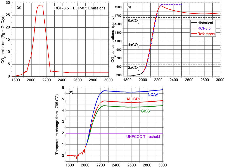
Figure 1. Temporal trajectories of: (a) Emission of CO2 in the RCP-8.5 and ECP-8.5 Reference scenario; (b) Historical, RCP- 8.5/ECP-8.5, and Reference CO2 concentrations simulated by the chemistry model; (c) Temperature change from 1765 for the reference case based on the values of climate sensitivity, aerosol forcing and thermal diffusivity obtained for the HADCRUT3, GISTEMP and NCDC temperature records.
lated by our carbon-cycle model [8] peaks at 1928 ppmv and then decreases due to natural carbon sinks to remain above 6 times the pre-industrial value out to year 3000. Similarly, the equivalent CO2 simulated by our model peaks at 2674 ppmv before declining slightly, but staying above 2400 ppmv. The concentrations of 30 other longlived GHGs are also calculated from their RCP-8.5 emissions by our chemistry model [8].
The CO2 emissions are based on the RCP historical and 8.5 future scenario. For the emissions from the beginning of the record until 2000, we divide the RCP historical emissions into Annex B and non-Annex B portions using the CDIAC country-specific fossil-fuel emissions database [9]. Since this database contains information only on emissions related to fossil-fuel use and cement production, and we do not have an analogous historical record to divide emissions related to land use into Annex B and non-Annex B countries, we have chosen not to include the historical emissions related to land use changes in our emissions total.
For the emissions beginning in 2000, we use the RCP- 8.5 emissions for both fossil fuel and land use. To insure a more continuous emissions record we turn the land-use forcing on over 10 years; including the full value of landuse forcing in 2000 results in a particularly discontinuous emissions record for non-Annex B. The RCP future scenarios are divided into geographic groups other than Annex B and non-Annex B. However, using the most recent year of data in the CDIAC database, we are able to determine that 99.06% of fossil-fuel CO2 emissions from the RCP’s “OECD90” group came from Annex B countries, and 80.60% of fossil-fuel CO2 emissions from the RCP’s “REF” group came from Annex B countries. Therefore, we compute the Annex B emissions from the RCP-8.5 scenario as 99.06% of the OECD90 emissions plus 80.60% of the REF emissions. While these percentages were obtained from fossil-fuel CO2 emissions, we apply them to the emissions of all long-lived GHG (LLGHG) species.
The additional species of LLGHGs contained in the RCP-8.5 emissions scenario are: CH4, N2O, CF4, C2F6, C6F14, HFC23, HFC32, HFC43-10, HFC125, HFC134a, HFC143a, HFC227ea, HFC245fa, SF6, CFC-11, CFC-12, CFC-113, CFC-114, CFC-115, CCl4, Methyl Chloroform, HCFC-22, HCFC-141B, HCFC-142B, Halon1211, Halon1202, Halon1301, Halon2402, CH3Br and CH3Cl.
For the emissions record beyond 2100, we use the ECP-8.5 emissions. Since the ECP-8.5 emissions are global totals with no geographic breakdown, we assumed the geographic partitions as percentages of world totals in years 2101 and after are equal to the partitions in year 2100.
The ECP-8.5 emissions record ends in 2500. For 2501- 3000, we assume constant emissions of each species for our reference case.
Based on a comparison of the emissions due to trade balance versus production [10], we multiply the emissions of Annex B countries by 1.12 in years 2008 and after, and the emissions of non-Annex B countries by 0.90 for the same years. To insure a more continuous emissions record, we phase these adjustments in over 10 years, starting in 1999.
We use the CICERO chemistry model [8] to convert the emissions input of LLGHGs to concentrations. We make several minor changes to the values of some coefficients to improve agreement with the RCP-8.5 concentrations, or to insure that in the mitigated case concentrations of LLGHGs other than carbon dioxide return to their pre-industrial values. Specifically, for carbon dioxide we change the fertilization factor from its default value of 0.287 to 0.077. We also change the timescale coefficient used in calculating the air-sea exchange from 9.06 years to 3.06 years. These changes allow us to better match the RCP-8.5 concentration peak (using the default values, our simulated carbon dioxide values ended up peaking a few hundred ppmv below the RCP-8.5 values, even when RCP-8.5 emissions were input exactly). However, for historical emissions, the calculated concentrations run about 22 ppmv too high as compared to observed. Therefore, we use historical concentrations prior to present, and calculated concentrations adjusted downward by about 22 ppmv for the future.
For methane we retain the same values for all the extinction coefficients, but we do not use the hydroxylradical feedback. We also use a value of 235.1 Tg/yr of natural methane emissions. For nitrous oxide we use an e-folding decay timescale of 86 years, and natural emissions of 15.2 Tg/yr. These changes better match our RCP trajectories in comparison with the concentration trajectories produced using the CICERO default values, while returning to the pre-industrial concentrations in the mitigated scenarios. For the other species we use the default parameters in the CICERO model. The concentrations are converted to forcings by the CICERO model [11].
For the emissions of sulfate, black-carbon and organiccarbon aerosols, we use the data from the RCP historical and 8.5 emissions scenario. For the scenario data, we partition the data into Annex B and non-Annex B regions by the same formula as used for the long-lived greenhouse gases. We also apply the trade adjustment to future emissions as described above.
The Simple Climate Model (SCM) that we use also requires the fractional split of each aerosol species between Northern and Southern Hemispheres. We calculate future Northern Hemisphere and Southern Hemisphere emissions based on the gridded data available from RCP. We use the CDIAC emissions for CO2 data as a proxy to determine the amount of aerosol emissions for Annex B countries in each hemisphere. For historical data, we use the fractional splits between hemispheres from [12] for sulfate aerosols, and [13-15] for black carbon and organic carbon.
We use the RCP historical and 8.5 scenario forcing record for tropospheric ozone. We partition the forcing between the hemispheres using the same percentages as for sulfate aerosols.
The historical solar record is based on the reconstructions of [16,17]. For future solar forcing, we assume there is no overall trend, and fit a sinusoidal curve to the last three sunspot cycles. We then extrapolate the solar record based on this fit.
We use a volcanic radiative forcing record [18], except we weight the radiative forcing by 0.6. This was done because using full-strength forcing causes unrealistically high negative temperature excursions in the years following volcanic eruptions, but using no volcanic forcing at all degraded agreement between simulated and observed ocean heat uptake. Post-2000 volcanic forcing is assumed to be zero.
3. Results
We calculate the change in global-average near-surface air temperature resulting from the emissions of long-lived GHGs and aerosols, as well as tropospheric ozone, landuse changes, historic volcanic eruptions and solar-irradiance variations, using our Simple Climate Model (SCM) [19]. The SCM was developed by Schlesinger in 1984, based on the model’s original formulation [20], and was used by Schlesinger and colleagues to simulate the globalmean temperature evolution for the different GHG scenarios of the IPCC 1990 report [21], for climate-impact studies [22-25], and greenhouse-policy studies [26-30]. A CD-based version of the SCM—the COuntry Specific Model for Intertemporal Climate (COSMIC) and its successor COSMIC2—has been distributed since 1997 to 130 requestors from 50 countries.
In a separate study we observationally estimated three SCM parameters [31]: 1) the equilibrium climate sensitivity, ∆T2x—the change in global-mean, equilibrium nearsurface temperature for a radiative forcing equivalent to a doubling of the pre-industrial CO2 concentration; 2) the total aerosol radiative forcing in reference year 2000, and 3) the ocean thermal diffusivity. These parameters were estimated for each of the three observational temperature datasets that begin in 1850: HADCRUT3 [32], and 1880: GISTEMP [33] and NCDC/NOAA [34]. The estimated climate sensitivity—1.45˚C, 1.61˚C and 1.98˚C for GISS, HADCRU and NOAA, respectively—is on the low side of the range given by the IPCC AR4 [35]. The resulting temperature changes from 1765 are presented in Figure 1(c). It is seen that the temperature change reaches the 2˚C threshold in 2050-2060, and thereafter rises to 4.4˚C, 4.9˚C and 5.8˚C for the parameter values based on the GISS, HADCRU and NOAA temperature datasets, respectively.
In our Fair Plan the GHG intensity—the amount of GHG emitted per unit of economic activity, relative to the Reference case—reduces from unity in 2015 to zero in 2065. This 50-year phase-out period for fossil-fuel emission mirrors the phase-out period proposed by the European Union [36]. As shown in Figure 2(a), the GHG intensity for Annex B countries decreases linearly, while that for the non-Annex B countries initially decreases more slowly than linearly and decreases more rapidly finally. We have chosen a cubic function of time for the latter such that, as shown in Figure 2(b), the total tradeadjusted CO2 emissions of the non-Annex B countries equals the total trade-adjusted CO2 emissions of the Annex B countries, 454.7 Pg of carbon (1667 Pg of CO2). Our accounting of global CO2 emissions includes an adjustment for international trade, since part of the increase in emissions in non-Annex B countries is due to production of goods that are consumed in Annex B countries. The CO2 emissions of the Annex B countries begin to decrease immediately, in 2016, but the CO2 emissions of the non-Annex B countries increase to 2042 before they too begin to decrease toward zero in 2065.
The resulting CO2 concentration, shown in Figure 2(c), peaks in 2060 at 529 ppmv, a value less than twice the pre-industrial concentration, and thereafter decreases to 362 ppmv in year 3000. The equivalent CO2 concentration—the amount of CO2 required to give the same radiative forcing as all the GHGs, including CO2—peaks at 626 ppmv in 2055 and declines to 363 ppmv in year 3000. Since the gases other than CO2 have virtually returned to
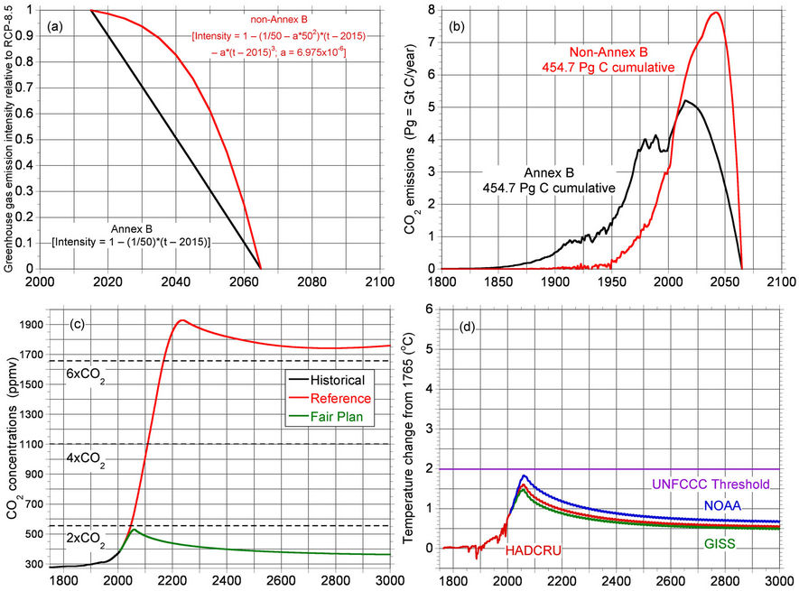
Figure 2. (a) Temporal evolution of the GHG emissions intensity for Annex B and non-Annex B countries during the phaseout period from 2015 to 2065; (b) Cumulative CO2 emissions by Annex B and non-Annex B countries; (c) CO2 concentrations calculated by our model for the Reference case and our Fair Plan emissions trajectory; (d) Global-mean near-surface temperature change from 1765 for our Fair Plan emissions trajectory and model parameters obtained for the HADCRUT3, GISTEMP and NCDC temperature records.
their pre-industrial concentration by this time, the equivalent CO2 concentration has essentially reduced to the actual CO2 concentration. The consequent temperature change calculated for the three observationally determined climate sensitivities, shown in Figure 2(d), peaks between 2058 and 2060 at 1.5˚C to 1.8˚C above pre-industrial, and thereafter decreases to between 0.5˚C to 0.7˚C in year 3000.
4. Discussion
Our Fair Plan reduces the emission of CO2 and the other GHGs to zero over the 50-year time period 2015 to 2065, equalizes the total emission of CO2 by the non-Annex B countries and the Annex B countries, keeps the maximum CO2 concentration below twice the pre-industrial value, and prevents the change in global-average nearsurface temperature from exceeding the 2˚C maximum warming threshold stipulated by the UNFCCC to “prevent dangerous human intervention in the climate system”.
Although the total, trade-adjusted emissions of CO2 by the Annex B countries and non-Annex B countries are equal under our Fair Plan, the per capita total emissions of the Annex B countries will be higher, since most of the world’s population lives in the non-Annex B countries. Given that non-Annex B countries may protest that their per-capita total emissions will be lower than the Annex B countries, we attempt to produce an emissions trajectory that equates Annex B and non-Annex B emissions on a per-capita basis rather than on a total emissions basis. This trajectory fails to meet the 2˚C maximum warming target.
In order to produce per-capita emissions estimates for the two groups, we use the RCP-8.5 emissions data as discussed above (including the trade adjustment). For historical population data previous to 1950 we use data from [37] and for population post-1950 and future population projections we use data from [38], employing the medium variant for the future projections. Since the country-specific numbers run only through 2100, we assumed the population of the world post-2100 is constant.
We show the cumulative per-capita emissions of the Annex B countries for our Fair Plan trajectory in Figure 3(a). We also compute the cumulative per-capita emissions for the non-Annex B countries using the RCP-8.5 emissions with no mitigation. The cumulative per-capita emissions for the non-Annex B countries are smaller than those for the Annex B countries out to the end of the ECP scenario in 2500, even when no mitigation is applied to the non-Annex B countries. Note that the RCP- 8.5/ECP-8.5 scenario contains a decline in CO2 emissions between 2150 and 2250; this decline is not applied by us. Assuming the medium scenario of population growth by [38], the cumulative per-capita emissions of the non-Annex B countries will remain smaller than our Fair Plan total for the Annex B countries if the non-Annex B emissions follow the RCP-8.5/ECP-8.5 curve.
Consequently, we run a scenario in our SCM whereby the Annex B countries follow our Fair Plan trajectory, but the non-Annex B countries follow the RCP-8.5/ECP- 8.5 trajectory with no mitigation. As shown in Figure 3(b), the 2˚C target is greatly exceeded, with maximum warming values of 3.4˚C - 4.5˚C obtained, depending on the climate sensitivity chosen.
While our Fair Plan does allow for greater per-capita emissions from the Annex B countries than the non-Annex B countries, the 2˚C target cannot be achieved for emissions trajectories that seek equality on a cumulative per-capita emissions basis, since the non-Annex B countries are not required to mitigate their emissions at all. The non-participation of non-Annex B countries will be politically unacceptable to many members of the Annex B group [4] and fails to stop the global warming from
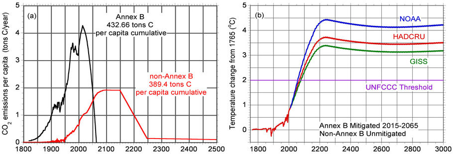
Figure 3. (a) Per capita emissions for Annex B and non-Annex B countries under which only Annex B countries follow our mitigation trajectories; (b) Global-mean near-surface temperature change from 1765 for the emissions trajectories in Figure 3(a).
exceeding the 2˚C threshold. Our Fair Plan, in contrast, requires participation from all countries but allows a slower initial mitigation trajectory for the non-Annex B countries, and meets the goal of limiting the global-mean temperature rise to below 2˚C. We believe our Fair Plan does the best job possible of addressing the concerns of both Annex B and non-Annex B nations while still meeting the 2˚C climate goal.
5. Acknowledgements
This work is funded by the United States National Science Foundation through grant ATM-0806155. Any opinions, findings, and conclusions or recommendations expressed in this material are those of the authors and do not necessarily reflect the views of the National Science Foundation.
REFERENCES
- United Nations, “United Nations Framework Convention on Climate Change,” 1992. http://unfccc.int/resource/docs/convkp/conveng.pdf
- Council of the European Union, “Presidency Conclusions,” 2005. http://register.consilium.europa.eu/pdf/en/05/st07/st07619-re01.en05.pdf
- United Nations, “Kyoto Protocol to the United Nations Framework Convention on Climate Change,” 1997. http://unfccc.int/resource/docs/convkp/kpeng.pdf
- Public Affairs Section, United States Embassy, Vienna, Austria, “Fact Sheet: United States Policy on the Kyoto Protocol,” 2001. http://www.usembassy.at/en/download/pdf/kyoto.pdf.
- United Nations, “Report of the Conference of the Parties on Its Sixteenth Session. Addendum Part Two: Action taken by the Conference of the Parties at Its Sixteenth Session,” 2010. http://unfccc.int/meetings/cancun_nov_2010/meeting/6266/php/view/reports.php
- K. Riahi, A. Gruebler and N. Nakicenovic, “Scenarios of Long-Term Socio-Economic and Environmental Development under Climate Stabilization,” Technological Forecasting and Social Change, Vol. 74, No. 7, 2007, pp. 887-935. doi:10.1016/j.techfore.2006.05.026
- M. Meinshausen, S. J. Smith, K. V. Calvin, J. S. Daniel, M. Kainuma, J.-F. Lamarque, K. Matsumoto, S. A. Montzka, S. C. B. Raper, K. Riahi, A. M. Thomson, G. J. M. Velders and D. van Vuuren, “The RCP Greenhouse Gas Concentrations and Their Extension from 1765 to 2300,” Climatic Change, Vol. 109, No. 1-2, 2011, pp. 213-241. doi:10.1007/s10584-011-0156-z
- J. S. Fuglesvedt and T. Berntsen, “A Simple Model for Scenario Studies of Changes in Climate. Version 1.0,” CICERO, Oslo, 1999.
- T. A. Boden, G. Marland and R. J. Andres, “Global, Regional and National Fossil-Fuel CO2 Emissions,” Carbon Dioxide Information Analysis Center, Oak Ridge, 2011.
- G. P. Peters, J. C. Minx, C. L. Weber and O. Edenhofer, “Growth in Emission Transfers via International Trade from 1990 to 2008,” Proceedings of the National Academy of Sciences, Vol. 108, No. 21, 2011, pp. 8903-8908. doi:10.1073/pnas.1006388108
- G. Myhre, E. J. Highwood, K. P. Shine and F. Stordal, “New Estimates of Radiative Forcing Due to Well Mixed Greenhouse Gases,” Geophysical Research Letters, Vol. 25, No. 14, 1998, pp. 2715-2718. doi:10.1029/98GL01908
- S. J. Smith, J. van Aardenne, Z. Klimont, R. Andres, A. C. Volke and S. Delgado Arias, “Anthropogenic Sulfur Dioxide Emissions 1850-2005,” Atmospheric Chemistry and Physics, Vol. 11, 2011, pp. 1101-1116. doi:10.5194/acp-11-1101-2011
- T. C. Bond, E. Bhardwaj, R. Dong, R. Jogani, S. Jung, C. Roden, D. G. Streets and N. M. Trautmann, “Historical Emissions of Black and Organic Carbon Aerosol from Energy-Related Combustion, 1850-2000,” Global Biogeochemical Cycles, Vol. 21, 2007, Article ID: GB2018. doi:10.1029/2006GB002840
- S. D. Fernandes, N. M. Trautmann, D. G. Streets, C. A. Roden and T. C. Bond, “Global Biofuel Use, 1850-2000,” Global Biogeochemical Cycles, Vol. 21, 2007, Article ID: GB2019. doi:10.1029/2006GB002836
- A. Ito and J. Penner, “Historical Emissions of Carbonaceous Aerosols from Biomass and Fossil Fuel Burning for the Period 1870-2000,” Global Biogeochemical Cycles, Vol. 19, 2005, Article ID: GB2028. doi:10.1029/2004GB002374
- J. Lean, G. Rottman, J. Harder and K. Kopp, “SORCE Contributions to New Understanding of Global Change and Solar Variability,” Solar Physics, Vol. 230, No. 1, 2005, pp. 27-53. doi:10.1007/s11207-005-1527-2
- Y.-M. Wang, J. L. Lean and N. R. Sheeley, “Modeling the Sun’s Magnetic Field and Irradiance since 1713,” Astrophyical Journal, Vol. 625, No. 1, 2005, pp. 522-538. doi:10.1086/429689
- N. G. Andronova, E. V. Rozanov, F. Yang, M. E. Schlesinger and G. L. Stenchikov, “Radiative Forcing by Volcanic Aerosols from 1850 through 1994,” Journal of Geophysical Research, Vol. 104, No. D14, 1999, pp. 16807-16826. doi:10.1029/1999JD900165
- M. E. Schlesinger, N. G. Andronova, B. Entwistle, A. Ghanem, N. Ramankutty, W. Wang and F. Yang, “Modeling and Simulation of Climate and Climate Change,” In: G. Cini Castagnoli and A. Provenzale, Eds., Past and Present Variability of the Solar-Terrestrial System: Measurement, Data Analysis and Theoretical Models, IOS Press, Amsterdam, 1997, pp. 389-429.
- M. I. Hoffert, A. J. Callegari and C.-T. Hsieh, “The Role of Deep Sea Heat Storage in the Secular Response to Climatic Forcing,” Journal of Geophysical Research, Vol. 85, No. C11, 1980, pp. 6667-6679. doi:10.1029/JC085iC11p06667
- C. S. Bretherton, C. Smith and J. M. Wallace, “An Intercomparison of Methods for Finding Coupled Patterns in Climate Data,” Journal of Climate, Vol. 5, No. 6, 1992, pp. 541-560. doi:10.1175/1520-0442(1992)005<0541:AIOMFF>2.0.CO;2
- R. J. Lempert, M. E. Schlesinger, S. C. Bankes and N. G. Andronova, “The Impacts of Climate Variability on NearTerm Policy Choices and the Value of Information,” Climatic Change, Vol. 45, No. 1, 2000, pp. 129-161. doi:10.1023/A:1005697118423
- R. Mendelsohn, W. Morrison, M. E. Schlesinger and N. G. Andronova, “Country-Specific Market Impacts of Climate Change,” Climatic Change, Vol. 45, No. 3-4, 2000, pp. 553-569. doi:10.1023/A:1005598717174
- R. Mendelsohn, M. E. Schlesinger and L. Williams, “Comparing Impacts Across Climate Models,” Integrated Assessment, Vol. 1, No. 1, 2000, pp. 37-48. doi:10.1023/A:1019111327619
- R. Mendelsohn, M. E. Schlesinger and L. Williams, “The Climate Impacts of Sulfate Aerosols,” Integrated Assessment, Vol. 2, No. 3, 2001, pp. 111-122. doi:10.1023/A:1013319100965
- M. E. Schlesinger and X. Jiang, “Revised Projection of Future Greenhouse Warming,” Nature, Vol. 350, 1991, pp. 219-221. doi:10.1038/350219a0
- R. J. Lempert and M. E. Schlesinger, “Robust Strategies for Abating Climate Change,” Climatic Change, Vol. 45, No. 3-4, 2000, pp. 387-401. doi:10.1023/A:1005698407365
- R. J. Lempert and M. E. Schlesinger, “Climate-Change Strategy Needs to Be Robust,” Nature, Vol. 412, 2001, p. 375. doi:10.1038/35086617
- R. J. Lempert and M. E. Schlesinger, “Adaptive Strategies for Climate Change,” In: R. G. Watts, Ed., Innovative Energy Systems for CO2 Stabilization, Cambridge University Press, Cambridge, 2002, pp. 45-86. doi:10.1017/CBO9780511536038.003
- R. J. Lempert, N. Nakicenovic, D. Sarewitz and M. E. Schlesinger, “Characterizing Climate-Change Uncertainties for Decisionmakers,” Climatic Change, Vol. 65, No. 1-2, 2004, pp. 1-9.
- M. J. Ring, D. Lindner, E. F. Cross and M. E. Schlesinger, “Causes of the Global Warming Observed Since the 19th Century,” Atmospheric and Climate Sciences, 2012, under review.
- P. Brohan, J. J. Kennedy, I. Harris, S. F. B. Tett and P. D. Jones, “Uncertainty Estimates in Regional and Global Observed Temperature Changes: A New Dataset from 1850,” Journal of Geophysical Research, Vol. 111, 2006, Article ID: D12106. doi:10.1029/2005JD006548
- J. Hansen, R. Ruedy, M. Sato and K. Lo, “Global Surface Temperature Change,” Reviews of Geophysics, Vol. 48, 2010, Article ID: RG4004. doi:10.1029/2010RG000345
- T. M. Smith, R. W. Reynolds, T. C. Peterson and J. H. Lawrimore, “Improvements to NOAA’s Historical Merged Land-Ocean Surface Temperature Analysis,” Journal of Climate, Vol. 21, No. 10, 2008, pp. 2283-2296. doi:10.1175/2007JCLI2100.1
- G. C. Hegerl, F. W. Zwiers, P. Braconnot, N. P. Gillett, Y. Luo, J. A. M. Orsini, N. Nicholls, J. E. Penner and P. A. Stott, “Understanding and Attributing Climate Change,” In: S. Solomon, D. Qin, et al., Eds., Climate Change 2007: The Physical Science Basis. Contribution of Working Group I to the Fourth Assessment Report of the Intergovernmental Panel on Climate Change, Cambridge University Press, Cambridge.
- European Commission, “A Roadmap for Moving to a Competitive Low Carbon Economy in 2050,” 2011. http://eur-lex.europa.eu/LexUriServ/LexUriServ.do?uri=CELEX:52011DC0112:EN:NOT
- A. Maddison, “Statistics on World Population, GDP and Per Capita GDP, 1-2008 AD,” 2008. http://www.ggdc.net/MADDISON/oriindex.htm
- United Nations, “World Population Prospects: The 2010 Revision,” 2010. http://esa.un.org/wpp/unpp/panel_population.htm