Energy and Power Engineering
Vol. 5 No. 2A (2013) , Article ID: 30598 , 10 pages DOI:10.4236/epe.2013.52A001
The Two-Constant Cost Model and the Estimation of the Cost Performance Evolutions of the Proton Exchange Membrane Fuel Cell Power Generation
State Key Laboratory of Automotive Safety and Energy, Tsinghua University, Beijing, China
Email: zhfsbqq@sohu.com, pchpei@tsinghua.edu.cn
Copyright © 2013 H. F. Zhang, P. C. Pei. This is an open access article distributed under the Creative Commons Attribution License, which permits unrestricted use, distribution, and reproduction in any medium, provided the original work is properly cited.
Received January 31, 2013; revised March 1, 2013; accepted March 15, 2013
Keywords: Fuel Cell; Cost Performance; Lifetime; Degradation; Energy Efficiency; Operation Optimization
ABSTRACT
This paper aims at formulization and overview of the cost performance evolutions of proton exchange membrane (PEM) fuel cell power generation along with load and time. For this purpose, electricity-cost ratio (ECR) is proposed as the measuring parameter for the cost performance and a two-constant cost model is proposed to concisely describe the cost characteristic of the power generation as the opposite of a multi-constant cost model. Combination of the two-constant cost model and the ideal cell model developed recently produces an inclusive ECR equation that has three analytical expressions and thus allows of straight overviews of the cost performance evolutions in the working zones of the cells. The applications to real cells confirm the validity of the equation for operation optimization and technique evaluation of PEM fuel cells. And more insights into the cost performance evolutions are inferred by means of the equation to help promote the commercialization of PEM fuel cells.
1. Introduction
PEM fuel cells are well known as one of the promising green power generation devices, but estimation and optimization of their cost performance has remained an important subject concerning successful commercialization of them all along. As one of critical integrated commercial indexes, the cost performance of the cells should be provided with concise and inclusive calculating formulae. Because of long lack of the formulae, broad overviews of the cost performance evolutions as load magnitude and operating time have scarcely ever been provided for real cells of various specialties and multifarious costs throughout their entire lifetimes. Again, there have been few guides for operation optimization of the cells towards cost performance maximization.
Great efforts have made for estimation of the cost performance or other relevant parameters, and several arithmetics [1-4] have been proposed. But few of them can effectively satisfy the current need. Among others, the core reason may lie in that no cell characteristics and/or no cost characteristics are concisely reflected and adequately included in them. In order to reform them towards current aim, as many factors of the cost performance as possible should be fused together. Performance, degradation, lifetime and cost are known as the major four of the factors, thus parameterizations and fusions of them may constitute a logic process to the goal. Considering cell diversity and cost miscellaneousness, two new models may get indispensable to the parameterizations and fusions.
One of the models may be the ideal cell model. It should be so developed as to extract cell constants for unified cell specialty characterization. This assignment has been successfully finished in one of our last works [5] and results in a five-constant ideal cell with outlined working zone. The ideal cell model may well allow of the derivation of the expected formulae in company with the other model and its working zone may well support an overview of cost performance evolutions in the entire operating range. Partially because of little acquaintance with the cell commonness and operating range, previous works [1-4] may suffer from disunified cell specialties and limited operating states, and few efforts have been made for the overview.
The other model refers to an appropriate cost model that needs to be established in this work. With it simple and effective cost classification can be performed for the derivation of cost performance formulae. The cost model can be so developed as to extract cost constants that group cost items into species according to the commonness of cost items. In essence, the model is designed to serve a special purpose, i.e. to combine the classical cost management theory with the features of fuel cells. It may be different from previous cost models that inclined to cost structure [2,3,6,7] or other concerns [1,4,8]. Without proper cost classification taken into account, previous cost models may not well support the combination.
Since cell performance, degradation characteristic and operation lifetime have been well fused together based on the ideal cell model, this work is arranged to develop the cost model, to more fuse power generation cost and to give cost performance overviews of the cells. It is also prepared for our next work where a direct tool will be developed for operation optimization and cost performance maximization of PEM fuel cells. As the premise of this work, a proper measuring parameter for the cost performance should be adopted. For the current subject, power-specific cost [6-8] or area-specific cost [2] may be not the most appropriate, while cost-electricity ratio (electricity price) [1,3,4] or its reciprocal (ECR) may be worth considering.
2. Cost Models and the Choice
As have been elaborated in pioneering documents [1-4, 6-8], there may be too many cost items in PEM fuel cell power generation. Different cost items may have different dependences on time or other parameters, so it may be possible and necessary for parameterized calculation of the total cost to group them according to the common natures of cost items. Cost classification may relate to electricity supply paths available for the terminal user. In general, the terminal user can gain electricity by two paths, thus there are two cost classifications and two cost models.
2.1. Two-Constant Cost Model
As the first path, the user purchases the cell and fuel by himself, and then directly supply himself; this path may be applicable to transportation, portable and stationary power (of any scale) users. In the first path, the total cost would be composed of two parts: the constant cost and the variable cost.
In direct proportion to fuel consumption or accumulative output charge quantity, the variable cost mainly includes fuel cost and maintenance cost, etc. Independent of fuel consumption or accumulative output charge quantity, the constant cost would be the acquisition cost of the cell. The acquisition cost mainly refers to the sale price of the cell offset by an estimated recyclable value (the disposal value of the cells). The acquisition cost includes the design cost, the production cost, the gross profit gained by cell producer, the taxies placed on the cell and the freight, etc. The cell production cost mainly includes various material costs, labor cost, power cost and depreciation of fixed assets, etc.
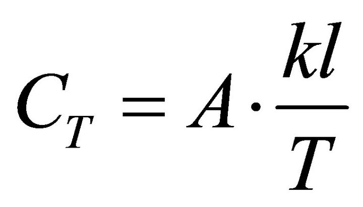
In the first path, the total cost may be calculated according to Formula (1). In Formula (1), l is the operating time or the actual service time of the cell, CT denotes the total cost, C and v are separately the constant cost measured in unit active area of the cells and the variable cost coefficient based on charge quantity, and the definite integral is the total charge quantity. Both C and v are called the cost constants.
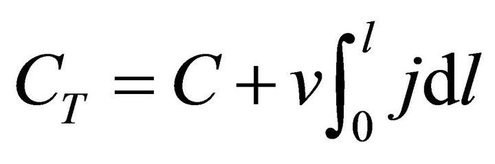 (1)
(1)
2.2. Multi-Constant Cost Model
The second path may be different from and associated with the first one. As the second path, the user can indirectly gain electrical energy supply from a power agent who purchases the cell and fuel; this path may be applicable to large-scale stationary power users. In the second path, the power agent would be an investor, so his earnings yield and charge policy would be involved in the cost calculation. The core of the problem is the consideration of the capital cost, one more cost item than those in the first path. This cost item is quite complex, as it has no simple fuel consumption dependences like those in the first path.
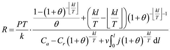
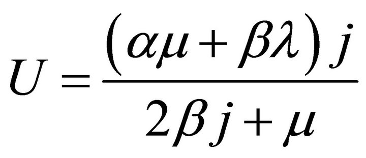
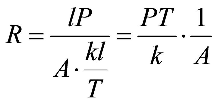
Assume that the investor gets the same fuel cell system at the same expense and by the same way with the terminal user in the first path, and consider such a charge policy: the electricity cost is charged periodically and equally, and once at the endpoint of each period; if the total apparent service time of the cells can be not divided exactly by the charge period, the residual is regarded as the last one normal period, but the electricity cost during the residual apparent service time is charged in the proportion of the residual apparent service time to one charge period at the endpoint of the last period. Treat the electricity cost as an annuity is done, then the total cost can be expressed as Formula (2). See Appendix for detailed derivation.
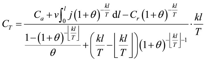 (2)
(2)
where, θ is the earnings yield during a charge period T; k is the ratio of the apparent service time to the actual service time of the cells (for example, if the actual service time of the cells is 8 hours per day, then k = 24/8 = 3); 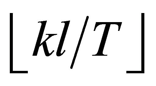 is an integral number not more than kl/T; Ca and Cr are the acquisition cost and the estimated recyclable value of the cells measured in unit active area, respectively, and Ca – Cr = C; the implications of other symbols are the same with in Formula (1).
2.3. The Choice of Cost Model
By comparing Formulae (1) and (2), the second cost classification may lead to more cost constants than the first one. Apparently, the total costs in the two paths are different, but the real expenses of a terminal user in the two paths may be the same in nature. In economic essence, the user seemingly pays the additional interest in the second path, while the interest essentially corresponds to the opportunity cost that is paid by the user for his purchase in the first path.
Because of high complexity of the calculation of total cost, the multi-constant cost model may make concise parameterization of the maximum cost performance almost impossible. Since total costs in the two models are equivalent in nature for a terminal user, this is to say, the opportunity cost reflected in the second path has actually been included in the total cost in the first path. We choose the first model for the following cost performance formulation.
The second model may lay much stress on return on capital and make a simple problem complicated. The same shortage also exists in some of previous cost models [1,2,4]. Besides, because of more parameters involved in the calculation of the total cost, it may become more difficult to combine them with the ideal cell model. Moreover, the operating time of the cells was measured in years to cater for annuity calculation, which may impair the practicability of the models more or less.
3. Formulation of Cost Performance
3.1. Parameter for Cost Performance
A proper parameter should be carefully selected to measure the cost performance. Power-specific cost [6-8] or area-specific cost [2] was frequently used to evaluate PEM fuel cells or their components. However, for the comprehensive quantitative estimation of the cost performance of PEM fuel cells, ECR may be more proper in cost-benefit principle. The reciprocal of ECR, cost-electricity ratio [1,3,4], may be acceptable likewise, but it may mainly serve to evaluate electricity price of the cells. In this work and the next, ECR is adopted as it may be more competent for operation optimization of the cells based on cost performance maximization.
3.2. ECR Basic Expression
PEM fuel cells are used to provide electrical energy, so the electrical energy would be the product of the power generation. Thus, bearing an analogy to the benefit-cost ratio of the production using a machine, the ECR of fuel cell power generation refers to the ratio of the total electrical energy provided by the cells to the total cost needed for the electrical energy.
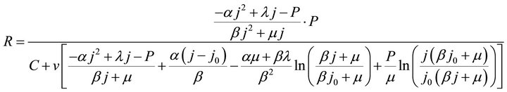
According to the definition, in the constant-power mode, the ECR of the fuel cell power generation can be expressed as Formulae (3) and (4) separately according to the twoand multi-constant cost models. Formulae (3) and (4) are separately called the first and second ECR basic expressions in which R denotes ECR and P denotes power density. Here, the second ECR basic expression is given only for a reference
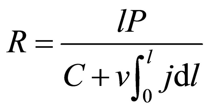 (3)
(3)
 (4)
(4)
A comparison between the first ECR basic expression and the basic expression for the average energy efficiency given in our last work [9] may well reveal the close connection between the average energy efficiency and the ECR. It may be indicated that an internal fusion of average energy efficiency and cost items is required for the ECR calculation, while the external fusion in which the average energy efficiency was included as an independent parameter [1,3] may not be the most appropriate treatment.
3.3. ECR Equations
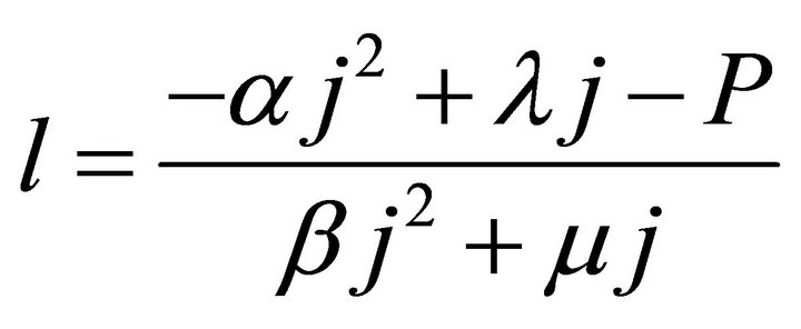
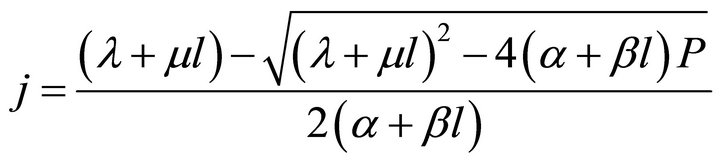
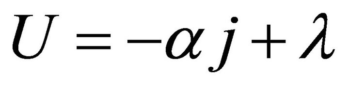
The ECR first basic expression can be unfolded as the average energy efficiency basic expression has been done [9]. To get the ECR basic expression manifested, the relationship between l and j should be firstly obtained, as given in Formula (5) or (6). It is derived by jointly solving the cell and load characteristic equations according to the ideal cell model. See our recent works [5,9] for details of the two characteristic equations.
 (5)
(5)
 (6)
(6)
In Formulae 5 and 6, U is cell voltage; α, λ, β and μ are cell characteristic constants: known as the polarization constants, the former two are the slope and the intercept of the linear part of the initial steady-state polarization (SSP) curve of the cells, and known as the degradation constants, the latter two are the change rates with time of the slope and the intercept; β and μ are not zero at the same time.
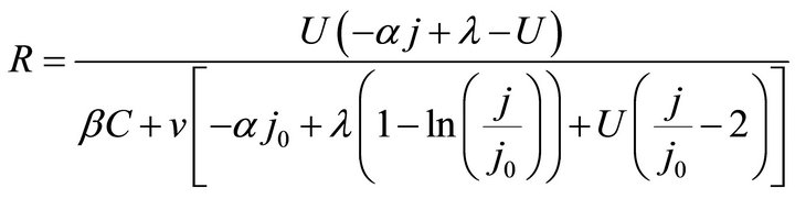
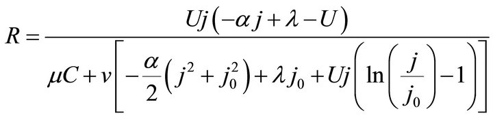
Substituting Formula (5) or (6) into Formula (3) gives three ECR formulae as shown in Formulae (7)-(9), corresponding to three different kinds of cell degradation characteristics. Formulae (7)-(9) are all called the ECR equation that comprehensively describe the ECR evolutions of PEM fuel cells as cell voltage, current density, load magnitude, operating time, cell initial performance, cell degradation parameters and cost characteristics of the power generation.
when 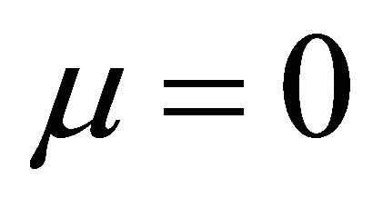 and
and ,
,
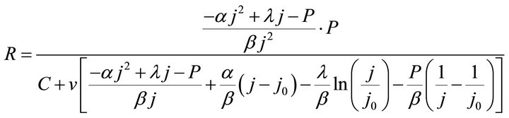 (7)
(7)
when  and
and ,
,
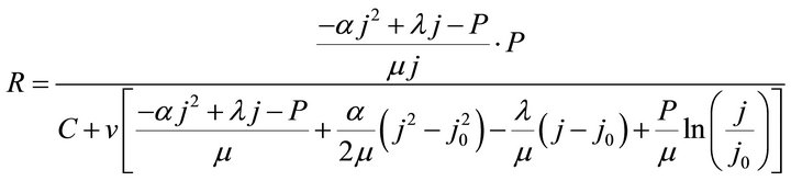 (8)
(8)
when  and
and ,
,
 (9)
(9)
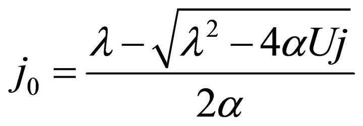
In Formulae (7)-(9), j0 denotes the initial operating current density given as:
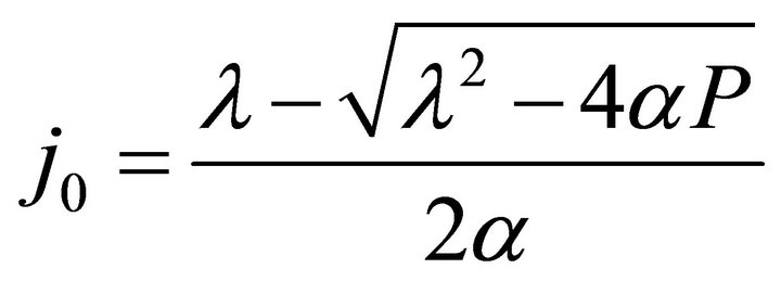 (10)
(10)
3.4. The Application Range
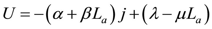
According to our recent works [5,9], the working zone may well define the whole operating range of a cell, so it may just be the application range of the ECR equation. In j/U plane, the working zone is an enclosed area by the initial SSP curve, the final SSP curve or the absolute lifetime end-curve, the relative lifetime end-curve and the j = 0 line. The former two curves are proximately represented separately by Formulae (11) and (12), and the third curve has three analytic expressions as given in Formulae (13)-(15), depending on different cell degradation characteristics. In Formula (12), La denotes the absolute lifetime of the cells.
 (11)
(11)
 (12)
(12)
when  and
and ,
,
 (13)
(13)
when  and
and ,
,
 (14)
(14)
when  and
and ,
,
 (15)
(15)
The working zone may be further divided by the critical load curve (or the minimum relative load curve) into two subzones including the absolute lifetime zone and the relative lifetime zone. No matter what the degradation characteristics of the cells are, the critical load curve can be represented with Formula (16).
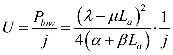 (16)
(16)
where, Plow is the critical load power density.
3.5. The Transplantability
Although the ECR equation is derived based on the ideal cell model in company with the two-constant cost model, it can be translated to a diversity of real cells. This is done through regularizing real cells with the ideal cell as prototype to formally revise real cells. There may exist some error in the regularization, but such a revision treatment may greatly facilitate the ability of the equation. See our recent work [5] for details of the revisions.
4. Overviews of Cost Performance Evolutions
4.1. ECR Contour Equation
On account of load power density contained, the ECR equation like Formulae (7)-(9) may go against straight exhibition of the ECR evolutions. For this reason, Formulae (7)-(9) are converted into their second form, as shown in Formulae (17)-(19), by substituting 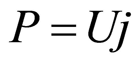 into them. Correspondingly, Formula (10) is turned into Formula (20).
when  and
and ,
,
 (17)
(17)
when 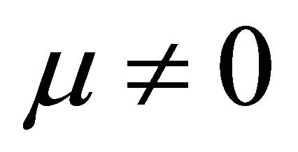 and
and ,
,
 (18)
(18)
when  and
and ,
,
 (20)
(20)
In j/U plane, Formulae (17)-(19) can present themselves as an ECR contour plot: the points of the same ECR constitute an equal ECR curve, and a series of equal ECR curves add up to an ECR contour distribution map. So, Formulae (17)-(19) may also be called the ECR contour equation, the second form of the ECR equation.
4.2. ECR Distributions
Similar to the treatment of the energy efficiency evolutions [9], the ECR evolutions can also been straight exhibited in j/U plane. This is done with the working zone as the medium, and results in the ECR distributions by drawing the ECR contours at regular intervals in the working zone. Again, the deconvolutions of the working zone by load curves and SSP curves may assist in analyzing ECR distributions and observing ECR evolutions.
Some distributions are displayed as examples in the next. In these distributions, curves abc, de, cd and bd are the initial SSP curve, the final SSP curve, the relative lifetime end-curve and the critical load curve, respectively; points a and e separately are the starting points of the initial and final SSP curves; points c and d separately are the intersection points of the initial and final SSP curves with the relative lifetime end-curve; point b is the intersection point of the critical load curve with the initial SSP curve; and dotted load curves at regular intervals of power density are also given.
4.3. Examples for Real Cells
The cost performance evolutions of real cells as operating time and load magnitude may be of interest. Here, we would display three examples as shown in Figures 1-3 separately for three real samples including two single cells and a 135-cell stack. Their working zones are all of ideally revised editions and the cell constant values are given in Table 1. See documents [5,10,11] for details of these samples. Without detailed cost information, both cost constants are roughly estimated at the same value for the three samples, as given in Table 1.
Given cell constants and cost constants, the ECR contour equation may be a two-variable function about cell voltage and current density. Thus there surely exists an operating point of the maximal ECR value in the working zone for any cell. This operating point is just the maximal cost performance (MCP) point, thus the ECR contour equation may contribute to find the MCP point for given cells and choose the optimal initial operating (OIO) point. The location of the MCP point may resolve the contradiction between efficient and full uses of the cells.
As seen from the ECR distributions in Figures 1-3, the MCP points of the three samples are located at almost the same site, around the endpoint of the critical load curve. The average efficiency for the three samples is calculated separately at around 38.00%, 36.35% and 38.25% according to the average efficiency formulae given in our last work [9], and the MCP is estimated separately at about 0.53, 0.61 and 0.57 kWh∙$−1 of ECR according to Figures 1-3. Obviously, the estimated MCP values may be much closer to one’s sensation of present commercial situation of PEM fuel cell power generation in comparison with the result, 0.04 $∙kWh−1 of electric price or 25
 (19)
(19)
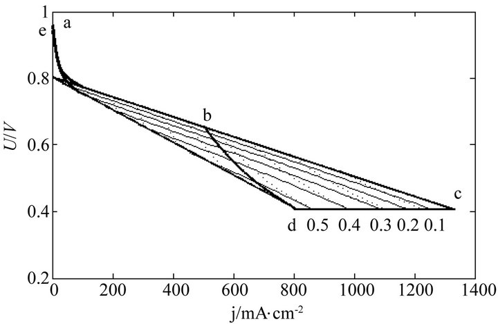
Figure 1. The ECR (kWh∙$−1) distribution of a real single cell in its ideally revised working zone. The dot curves are the load curves at 50 mW∙cm−2 intervals and the critical load power density is 329 mW∙cm-2.
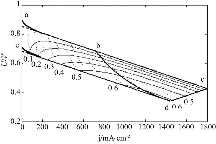
Figure 2. The ECR (kWh∙$−1) distribution of another real single cell in its ideally revised working zone. The dot curves are the load curves at 50 mW∙cm−2 intervals and the critical load power density is 492 mW∙cm-2.
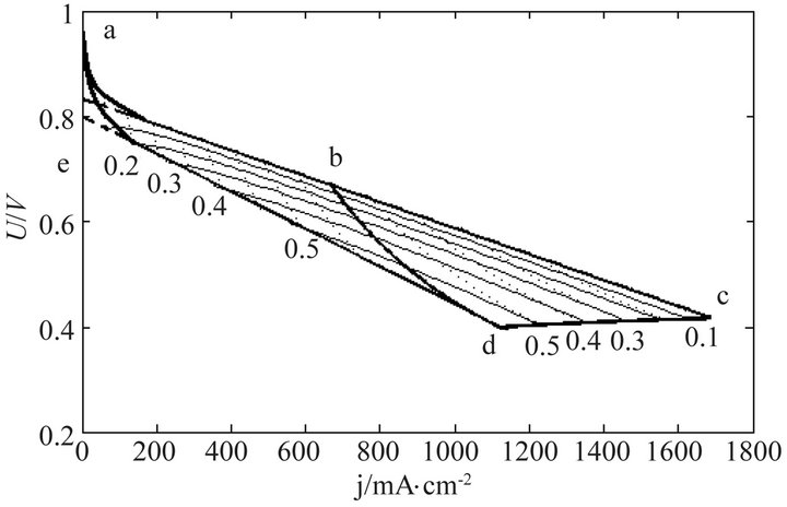
Figure 3. The ECR (kWh∙$−1) distribution of a real 150- cell stack in its ideally revised working zone. The dot curves are the load curves at 50 mW∙cm−2 intervals and the critical load power density is 449 mW∙cm-2. U denotes unit-cellaveraged voltage.
kWh∙$-1 of ECR, from other calculation model [3].
Move upstream along the critical load curve to the initial SSP curve, then the OIO points of the three samples
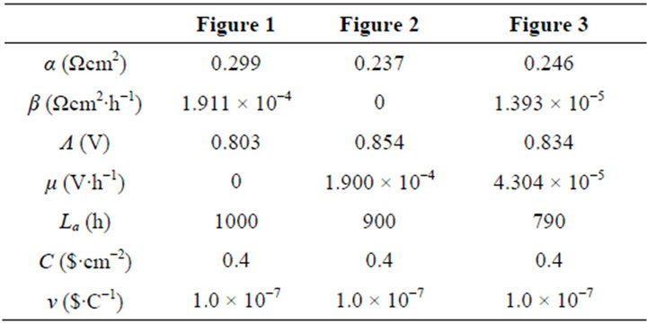
Table 1. The values of cell constants and cost constants in Figures 1-3.
can be located. As seen from Figures 1-3, the operating voltage at the OPO point is 0.66 V, 0.69 V and 0.67 V, respectively, for the three samples. These values coincide with the practice of PEM fuel cells on the selection of initial voltage. Avoidance of catalyst corrosion was once one of the considerations for the practice. Now it may be understood the practice seems motivated more inherently by economical consideration. It may also be seen from Figures 1-3 that the initial current density for each sample is located in the linear polarization region of the SSP curve, which may well support the fourth assumption about the ideal cell model [5].
5. Extended Discussion
Besides for operation optimization and cost performance comparison, the ECR equation may also serve to predict. Here, we take three ideal cells of long lifetime as samples to see the cost performance evolutions. The samples are of the totally same polarization characteristic and separately of three different kinds of degradation characteristics. Two levels of constant cost and two levels of variable cost coefficient in total are taken equally for each sample. See Table 2 for the values of the cell constants and cost constants.
Twelve ECR distributions in total are displayed in Figures 4-6. From them it may be seen that the MCP point doesn’t happen at the critical load curve and even not at the absolute or relative lifetime endpoint for the cells of long lifetime. From the ECR distribution changes with cell characteristic and cost characteristic displayed in Figures 4-6 and in company with the ECR equation, more insights can be inferred:
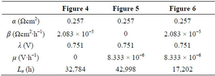
Table 2. The cell constant values in Figures 4-6.
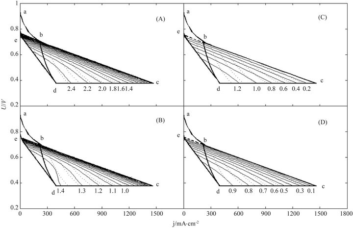
Figure 4. The ECR (kWh∙$−1) distributions of the first ideal cell under cost characteristics (A) C = 0.4 $∙cm−2 and v = 0.5 × 10⁻⁷ $∙C−1; (B) C = 0.4 $∙cm-2 and v = 1.0 × 10⁻⁷ $∙C−1; (C) C = 2.0 $∙m−2, v = 0.5 × 10⁻⁷ $∙C−1 and (D) C = 2.0 $∙cm−2 and v = 1.0 × 10⁻⁷ $∙C−1. The dot curves are the load curves at 50 mW∙cm−2 intervals and the critical load power density is 150 mW∙cm−2.
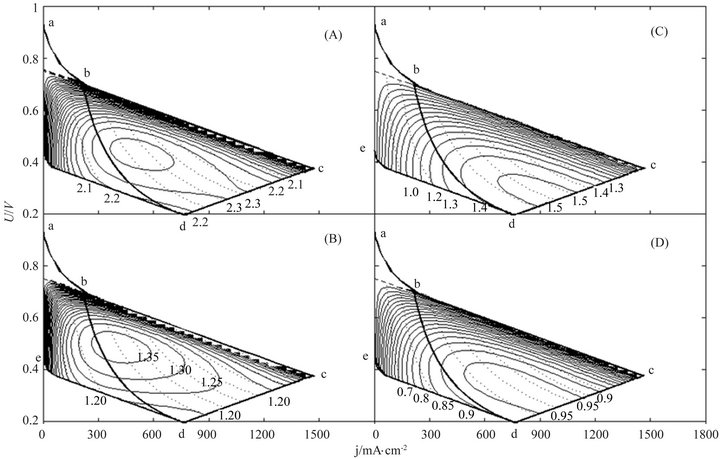
Figure 5. The ECR (kWh∙$−1) distributions of the second ideal cell under the same cost characteristics with the first one. The dot curves are the load curves at 50 mW∙cm−2 intervals and the critical load power density is 150 mW∙cm−2.
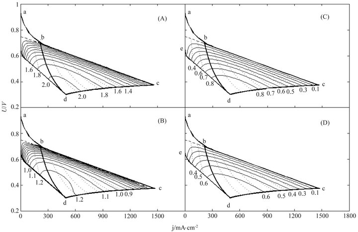
Figure 6. The ECR (kWh∙$−1) distributions of the third ideal cell under the same cost characteristics with the first one. The dot curves are the load curves at 50 mW∙cm−2 intervals and the critical load power density is 150 mW∙cm−2.
1) Improving cell performance (i.e. increasing λ and/or decreasing α, β and μ), lowering the power generation costs and selecting the optimum load power and operating time, would be the three ways to maximize the cost performance of the PEM fuel cell power generation and thus to successfully commercialize PEM fuel cells.
2) The cost performance of the PEM fuel cell power generation in a given cell would be not a constant but a variable depending on the load power density and the operating time. There surely exists a MCP point in the working zone of the cell, whose ECR value may quantitatively indicate the technical level of the cell.
3) The MCP point is jointly determined by the cell characteristic and the power generation cost characteristic, and it possesses three attributes: the maximum ECR value, the optimum load power and the optimal operating time. So the MCP point would indicate not only the best achievement of the PEM fuel cell power generation but also the conditions for the achievement.
4) The full level of the PEM fuel cell power generation technology does not require a too long absolute lifetime for some cells. In one of the sampled cases, about 25,000 hours may be enough. It can clearly be seen from Figure 5 that the maximum ECR of the PEM fuel cell power generation can be achieved as long as the absolute lifetime of the cell is as long as the optimal service time. Only in the case of the absolute lifetime less than the optimal operating time, the absolute lifetime of the cell may be worth increasing.
5) If there may exist a requirement for the ECR, the service time of the cell would be restricted, and this may lead to an economic lifetime of the cell. Different from other lifetime forms of the cell, the economic lifetime of the cell would be subjective, and it can be figured out according to the ECR equation, the cell characteristic equation and the requirement regarding the ECR.
6) A good PEM fuel cell recycle policy would be of great significance for the substantial commercialization of the PEM fuel cell power generation technology. A PEM fuel cell would have many recyclable components or materials of high value such as flow-field plate, noble metal etc. A circular use of the recyclable components and materials at an appropriate price would be in favor of the increase of the cost performance of the PEM fuel cell power generation.
7) Due to the variable cost, the influence of the constant cost on the cost performance of the PEM fuel cell power generation would be weakened greatly.
6. Remarks
In the derivation of the ECR equation, only the linear polarization region of the cells is taken into consideration. This treatment may be allowable. From the derivation of the ECR equation it may be understood the unfolding of the ECR basic expression will become more difficult if without this treatment. Although this treatment would produce error for the ECR calculation in the activation polarization region, it may seldom affect the determination of the MCP point. Intuitively, the MCP point may rarely occur in low load power range that corresponds to the activation polarization region. In the examples of ECR distribution in Section 5, distinct activation polarization regions are intentionally displayed to remind of the treatment. In quite a few real cells, the activation polarization region appears indistinct, which may more support this treatment as discussed in Section 4.3.
7. Conclusions
Cell performance, degradation characteristic, service lifetime, load magnitude and power generation cost are successfully fused into an organic whole for formulation of the cost performance of PEM fuel cells. There are two economically equivalent cost models in total for mathematical characterization of the total cost. But only one of them, the two-constant cost model, well suits the purpose of combination with the five-constant ideal cell model by virtue of conciseness. The combination produces an inclusive electricity-cost ratio (ECR) equation that has three analytical expressions.
The equation allows of straight overviews of the cost performance evolutions along with load and time as well as cell and cost in the working zones in the form of ECR distribution. And it can be translated to a diversity of real cells by formal revision of them. The applications to real cells confirm its validity for operation optimization and technique evaluation of PEM fuel cells. And it well accounts for the practical selection of the initial operating point of PEM fuel cells.
Any PEM fuel cell surely possesses an economically optimal operating endpoint where the ECR value may quantitatively indicate its technical level. The optimal operating end-point possesses three attributes: the maximum ECR value, the optimum load power and the optimal service time. It would indicate not only the best achievement of the PEM fuel cell power generation but also the conditions for the achievement. And the full level of the PEM fuel cell power generation technology does not require a too long absolute lifetime for some cells.
8. Acknowledgements
This paper has been supported by the National 973 Program (No. 2012CB215500) and the National 863 Programs of China (No. 2012AA053402, No. 2012AA053 402).
REFERENCES
- A. Kazim, “A Novel Approach on the Determination of the Minimal Operating Efficiency of a PEM Fuel Cell,” Renewable Energy, Vol. 26, No. 3, 2002, pp. 479-488. doi:10.1016/S0960-1481(01)00083-0
- K. Jayakumar, S. Pandiyan, N. Rajalakshmi and K. S. Dhathathreyan, “Cost-Benefit Analysis of Commercial Bipolar Plates for PEMFCs,” Journal of Power Sources, Vol. 161, No. 2, 2006, pp. 454-459. doi:10.1016/j.jpowsour.2006.04.128
- S. K. Kamarudin, W. R. W. Daud, A. Md. Som, M. S. Takriff and A. W. Mohammad, “Technical Design and Economic Evaluation of a PEM Fuel Cell System,” Journal of Power Sources, Vol. 157, No. 2, 2006, pp. 641-649. doi:10.1016/j.jpowsour.2005.10.053
- Y. Ma, G. G. Karady, A. Winston II, P. Gilbert, R. Hess and D. Pelley, “Economic Feasibility Prediction of the Commercial Fuel Cells,” Energy Conversion and Management, Vol. 50, No. 2, 2009, pp. 422-430. doi:10.1016/j.enconman.2008.09.009
- H. F. Zhang, P. C. Pei, X. Yuan and X. Z. Wang, “Regularization of the Degradation Behavior and Working Zone of Proton Exchange Membrane Fuel Cells with a Five-Constant Ideal Cell as Prototype,” Energy Conversion and Management, Vol. 52, No. 10, 2011, pp. 3189- 3196. doi:10.1016/j.enconman.2011.04.022
- I. Bar-On, R. Kirchain and R. Roth, “Technical Cost Analysis for PEM Fuel Cells,” Journal of Power Sources, Vol. 109, No. 1, 2002, pp. 71-75. doi:10.1016/S0378-7753(02)00062-9
- H. Tsuchiyaa and O. Kobayashib, “Mass Production Cost of PEM Fuel Cell by Learning Curve,” International Journal of Hydrogen Energy, Vol. 29, No. 10, 2004, pp. 985-990. doi:10.1016/j.ijhydene.2003.10.011
- W. P. Teagan, J. Bentley and B. Barnett, “Cost Reductions of Fuel Cells for Transport Applications: Fuel Processing Options,” Journal of Power Sources, Vol. 71, No. 1-2, 1998, pp. 80-85. doi:10.1016/S0378-7753(97)02796-1
- H. F. Zhang, P. C. Pei, M. C. Song and D. P. Zhang, “A Volt-Ampere Method to Estimate the Energy Efficiency Evolutions of Proton Exchange Membrane Fuel Cells along with Load and Time,” Energy Power Engineering, in Press.
- D. Liu and S. Case, “Durability Study of Proton Exchange Membrane Fuel Cells under Dynamic Testing Conditions with Cyclic Current Profile,” Journal of Power Sources, Vol. 162, No. 1, 2006, pp. 521-531. doi:10.1016/j.jpowsour.2006.07.007
- M. Prasanna, E. A. Cho, T. H. Lim and I. H. Oh, “Effects of MEA Fabrication Method on Durability of Polymer Electrolyte Membrane Fuel Cells,” Electrochimica Acta, Vol. 53, No. 16, 2008, pp. 5434-5441. doi:10.1016/j.electacta.2008.02.068
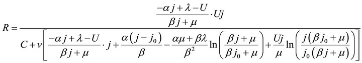
Appendix
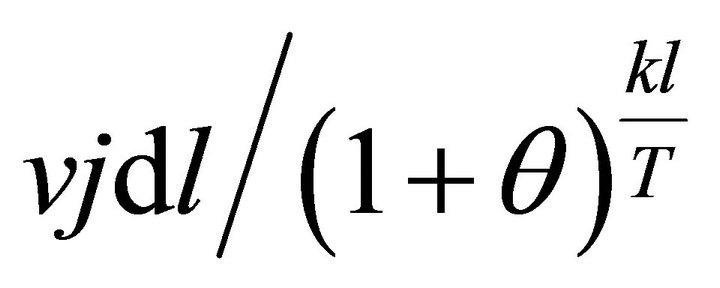
With A denoting the charge quantity in a whole charge period at the endpoint of each period, the total cost and the ECR can be expressed separately as Formulae (A.1) and (A.2) in the second electricity supply path.
 (A.1)
(A.1)
 (A.2)
(A.2)
According to the charge policy, the total present value of the costs paid by the user can be expressed as in Formula (A.3). The first term represents the sum of present value of the cost paid in every normal charge period at each side of equal sign, and the second term represents the present value of the cost paid in the residual apparent service time.
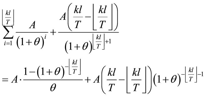 (A.3)
(A.3)
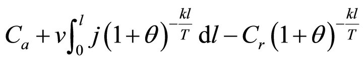
The total present value of the capitals committed by the investor can be expressed as Formula (A.4). The first term represents the present value of the acquisition cost of the cell, the second term represents that of variable cost, gained from the present value differential,
 , and the third term represents that of estimated recyclable value of the cell.
 (A.4)
(A.4)
According to cost management principle, the total present value of the costs paid by the user should be equal to the total present value of the capitals committed by the investor, thus the charge quantity in a whole charge period can be expressed as Formula (A.5):
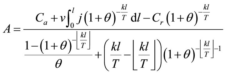 (A.5)
(A.5)
Substituting Formula (A.5) into Formula (A.1) gives Formula (2) and into Formula (A.2) gives Formula (4).