Advances in Pure Mathematics
Vol.09 No.04(2019), Article ID:91715,13 pages
10.4236/apm.2019.94014
An Expanded Optimal Control Policy for a Coupled Tanks System with Random Disturbance
Sie Long Kek1, Sy Yi Sim2, Chuei Yee Chen3
1Department of Mathematics and Statistics, Universiti Tun Hussein Onn Malaysia, Pagoh, Malaysia
2Department of Electrical Engineering Technology, Universiti Tun Hussein Onn Malaysia, Pagoh, Malaysia
3Department of Mathematics, Universiti Putra Malaysia, Serdang, Malaysia

Copyright © 2019 by author(s) and Scientific Research Publishing Inc.
This work is licensed under the Creative Commons Attribution International License (CC BY 4.0).
http://creativecommons.org/licenses/by/4.0/


Received: March 4, 2019; Accepted: April 8, 2019; Published: April 11, 2019
ABSTRACT
In this paper, an expanded optimal control policy is proposed to study the coupled tanks system, where the random disturbance is added into the system. Since the dynamics of the coupled tanks system can be formulated as a nonlinear system, determination of the optimal water level in the tanks is useful for the operation decision. On this point of view, the coupled tanks system dynamics is usually linearized to give the steady state operating height. In our approach, a model-based optimal control problem, which is adding with adjusted parameters, is considered to obtain the true operating height of the real coupled tanks system. During the computation procedure, the differences between the real plant and the model used are measured repeatedly, where the optimal solution of the model used is updated. On this basis, system optimization and parameter estimation are integrated. At the end of the iteration, the iterative solution approximates to the correct optimal solution of the original optimal control problem, in spite of model-reality differences. In conclusion, the efficiency of the approach proposed is shown.
Keywords:
Expanded Optimal Control, Coupled Tanks System, Model-Reality Differences, Iterative Solution, Adjusted Parameters

1. Introduction
A coupled tanks system, which consists of a joint of two tanks together through pipes in order to reserve water at the operating height level, is an important study in the control engineering and process industries [1] . The applications of the coupled tanks system have been widely used in the real-world process, for example, petrochemical, waste-water treatment, and purification [2] [3] . Essentially, the coupled tanks modeling provides a configurable process control experiment to engineers and researchers such that a wide array of modeling and control-related laboratory works on liquid control can be performed in advance [1] .
Theoretically, the dynamics of the coupled tanks system is formulated into a system of differential equations. The inflow and the outflow of the coupled tanks system are monitored in a simulation way in which the balance between the change rate of the water height level and the water flow in and out can be measured precisely. In addition to this, the water flow rate shall be controlled such that the equilibrium of the steady state along the operating height level is established. In literature, there are many studies on this steady state of the water level that are carried out. See for more detail in [4] [5] [6] .
In practice, the experimental works on the coupled tanks system, which cover the inflow and the outflow, are affected by some disturbances, such as inaccuracy of apparatus, man-made error and unfamiliar skill, and would give the inappropriate results [7] . Due to these reasons, the steady-state of the operating height level in the coupled tanks system is not easy to be addressed [8] . Therefore, approximating the operating height level in the coupled tanks system as accurately as possible attracts the interest of engineers and researchers.
Therefore, in this paper, an expanded optimal control policy, which takes into account different structures and parameters [9] [10] [11] , is proposed for determining the steady-state of the operating height level of a couple tanks system with random disturbance. In our approach, the adjusted parameters are added to the model used. Accordingly, the expanded optimal control model is further defined [12] [13] [14] . Especially, the optimal control policy, which is known as the expanded optimal control policy, is designed for solving the expanded optimal control model iteratively. On this basis, an illustrative example of the coupled tanks system, which is disturbed by the random noise, is presented. As a result, the optimal operating height level of the coupled tanks system is determined. Hence, the efficiency of the approach proposed is highly recommended.
The structure of the paper is organized as follows. In Section 2, the problem on the coupled tanks system is described, where the related mathematical model is formulated. In Section 3, the expanded optimal control model, which is added the adjusted parameters into the model used, is introduced. From the iterative calculation, the expanded optimal control policy, which determines the optimal operating height level in the coupled tanks system, is obtained. In Section 4, the illustrative example of the coupled tanks system is discussed. The result shows the application of the approach proposed. Finally, some concluding remarks are made.
2. Problem Statement
Consider that two tanks are joined to be the coupled tanks system [3] [4] [5] [6] . The system states are the water level H1 in Tank 1 and the water level H2 in Tank 2. The control input is the pump flow rate and the variable to be controlled is the second state, which is the water level H2, with disturbances that are caused by variations in the rate of flow out of the system by Valve B or by changes in Valve C. Hence, a mathematical model shall be built for each of the tank water levels. Figure 1 shows the system plant that is determined by relating the flow into the tanks to the flow leaving the valve at the tank bottom.
The flow balance equation for Tank 1 is given by
(1)
where is the cross-sectional area of Tank 1, is the flow rate of water from Tank 1 to Tank 2 through Valve B. While, for Tank 2, the flow balance equation is given by
(2)
where is the cross-sectional area of Tank 2, is the flow rate of water out of Tank 2 through Valve C. The system plant comes from the two flow balances and the nonlinear equations for flows through the valves.
With the assumption that the valves are ideal orifice, the flows through the valves will be related to the water levels in the tanks by the following expressions:
and (3)
where and are, respectively, the cross sectional areas of the orifice at Valves B and C, and and are the discharge coefficients of Valves B and C, respectively. These coefficients take into account all fluid characteristics, losses and irregularities in the system to make the two sides of (1) and (2) balance. The gravitational constant is given by g = 9.80 m/s2. In addition to this, the two flow balances for ideal valves, which are given by (1) and (2), are rewritten by
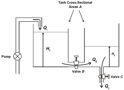
Figure 1. A coupled tanks system.
(4)
(5)
Here, (4) and (5) describe the coupled tanks system dynamics in the nonlinear manner with ideal equations for the valves. In practice, the cross sectional area is given by the dimensions of the valve and the flow channel, which could be more complicated.
Denote with as the heights of water level in the tanks, is the control input, and let
and . (6)
In presence of the random disturbances, the system plant dynamics in (4) and (5) is rewritten as
(7)
(8)
where is the Gaussian random variable with zero mean and covariance . Hence, this problem of controlling the water level in Tank 2 can be formulated as an optimal control problem, which is referred to as Problem (P), given below [11] [12] :
Problem (P): Find the optimal control input u, which is the flow rate, to minimize the cost function
(9)
subject to the system dynamics (7) and (8) with the output measurement , where and are the steady states of the value, r is the positive weight coefficient, is the initial time and is the fixed terminal time.
Notice that the structure of Problem (P) is complex and nonlinear. Solving Problem (P) would be computational demanding. However, the optimal solution of Problem (P) could be obtained through solving its simplified model, which is referred to as Problem (M), given by
(10)
with
, , , (11)
where and are the steady states of the value, whereas, is the adjustable parameter.
Refer to this simplified model, it is highlighted that the aim of adding the adjustable parameter into the model used in Problem (M) is to measure the differences between the system plant and the linear model used repeatedly. By virtue of this, the optimal solution of the model used could be updated in order to approximate the correct optimal solution of Problem (P), in spite of model-reality differences [9] - [14] .
3. System Optimization with Parameter Estimation
Now, refer to the cost function in (9) or (10), setting the weighting coefficient matrices Q and R, and the state transition matrix A and the control coefficient matrix B, respectively, to be
, , , . (12)
Let represents the system dynamics function of the coupled tanks system, that is,
(13)
. (14)
Let us define an expanded optimal control problem, which is referred to as Problem (E), given by
(15)
where and are introduced to separate the control variable and the state variable in the optimization problem from the respective signals in the parameter estimations problem, and denotes the usual Euclidean
norm. The terms and with and
are introduced to improve the convexity and to facilitate the convergence of the resulting iterative algorithm. It is important to note that the algorithm is designed in such a way that the constraints and are satisfied due on the termination of iterations, assuming convergence is achieved. The state constraint and the control constraint are used for the computation of the parameter estimation and the matching scheme, while the corresponding state constraint and control constraint are reserved for optimizing the linear model-based optimal control problem. Hence, system optimization and parameter estimation are mutually interactive.
3.1. Necessary Conditions
Define the Hamiltonian function by
(16)
where is the Lagrange multiplier. Then, the augmented cost function for the cost function in (15) becomes
(17)
where and are the appropriate multipliers to be determined later.
Applying the calculus of variation [14] [15] [16] , the following necessary conditions for optimality are obtained.
a) Stationarity:
(18)
b) Co-state equation:
(19)
c) State equation:
(20)
d) Output equation:
. (21)
e) Boundary condition:
and are given. (22)
f) Adjustable parameter equation:
(23)
g) Multiplier equations:
, (24)
. (25)
h) Separable variables:
, , (26)
with and .
3.2. Modified Optimal Control Problem
From the necessary conditions (18)-(22), a modified optimal control problem, which is referred to as Problem (MM), is defined by
(27)
with the specified and , where the boundary conditions and are given.
3.3. Optimal Control Law
The optimal control law for Problem (MM), which is known as the expanded optimal control policy, is a feedback control [9] - [14] . This control law is stated in the following theorem.
Theorem 1 (Expanded optimal control policy): Assume that the expanded optimal control policy exists. Then, this optimal control law is the feedback control law for Problem (MM), given by
(28)
where
(29)
(30)
(31)
(32)
with the boundary conditions and , and
Proof: From the necessary condition (18), the optimal control is written by
. (33)
Applying the sweep method [15] [16] ,
(34)
into (33), after some algebraic manipulations, the feedback control law (28) is obtained, where (29) and (30) are satisfied.
Also, substitute (34) into the costate equation (19) to yield
(35)
Differentiating both sides (34) with respect to t gives
(36)
Notice that (35) and (36) are equivalent. That is,
(37)
Then, consider the state equation (20) and the feedback control (28) in (37). After doing some algebraic manipulations by taking into account (29) and (30), then (31) and (32) are satisfied. This completes the proof.
Now, taking (28) into (20), the state equation becomes
(38)
with the output measurement
. (39)
3.4. Iterative Procedure
From the discussion above, the calculation procedure is summarized as an iterative algorithm given below.
Algorithm 1: Iterative algorithm
Data and f.
Step 0 Compute a nominal solution. Assuming that , compute and , respectively, from (30) and (31), and solve Problem (M) defined in (10) to obtain . Set , , , , for .
Step 1: Compute the parameter from (23). This is called the parameter estimation step.
Step 2: Compute the multipliers and from (24) and (25).
Step 3: Using and , solve Problem (MM) defined in (27) by using the result that is presented in Theorem 1. This is called the system optimization step.
1) Solve (32) forward to obtain and solve (29) to obtain .
2) Use (28) to obtain the new control .
3) Use (38) to obtain the new state .
4) Use (34) to obtain the new costate .
5) Use (39) to obtain the new output .
Step 4: Test the convergence and update the optimal solution of Problem (P). In order to provide a mechanism for regulating convergence, a simple relaxation method is employed:
(40)
where are scalar gains. If within a given tolerance, stop; else set , and repeat the procedure staring from Step 1.
Remarks:
a) The nominal solution can be the optimal solution that is obtained from the standard linear quadratic regulator (LQR) optimal control problem.
b) The off-line computation for solving (30) and (31) is done at Step 0 before the iteration begins with assuming and .
c) The numerical scheme for solving the ordinary differential equations of and can be used.
d) The relaxation method given in (40) establishes a matching scheme for the updating of the iterative solution.
4. Result and Discussion
For the numerical illustration, the physical parameters of the coupled tanks system are shown in Table 1 [4] . The steady states of the value are set at and , while the weight of coefficient is r = 1 and the time given is .
Follow from this, the algorithm proposed is applied to obtain the optimal operating height level in the coupled tanks system. For doing this task, the algorithm proposed is implemented in the MATLAB 2016 R1 environment in Window 8.1 Pro with the processor 2.10 GHz and the 64-bit operating system. Refer to Table 1, the system parameters used are calculated and given as follow:
, and .
The simulation result is shown in Table 2. The final cost gives a smaller value than the original cost, which saves about 0.039 percent of the original cost spent.
Figure 2 shows the trajectory of control input for the coupled tanks. The control input reduces its value dramatically from 3.33 units and then increases gradually after 0.2 seconds. It takes 0.6 seconds to converge to the steady state value . This behavior of the control input indicates that the flow rate, which is pumped into Tank 1 for the first 0.2 second, is moved into Tank 2 and reaches at the steady state after 0.8 seconds.
In addition to this, the water in Tank 2 is controlled at the steady-state value units as shown in Figure 3 and Figure 4. It can be seen that the original state trajectory is disturbed by the random disturbances. Nonetheless, the expected state trajectory, which is measured from the origin, is increased obviously in such a way that controlling the steady-state value of the water level in the second tank is made.

Table 1. Physical parameters of coupled tanks system.
Table 2. Simulation result.

Figure 2. Control trajectory.

Figure 3. State trajectory.
Figure 5 shows the stationary condition of the optimality. It verifies that the iterative algorithm proposed is efficient and the final solution is the optimal solution. As a result, the iterative algorithm proposed is applicable to making the decision on the operating height of the coupled tanks system.

Figure 4. Output trajectory.

Figure 5. Stationary condition of optimality.
5. Concluding Remarks
The use of the expanded optimal control policy in determining the operating height level in the coupled tanks system was discussed in this paper. The special feature of this expanded optimal control policy is that the model used, which is a linear model, has a different structure compared to the original problem, which is a nonlinear model. By adding the adjusted parameters into the model used, the differences between the model used and the original model could be measured iteratively. As a result, the flow rate of the coupled tanks system is controlled and the operating height level is achieved, in spite of model-reality differences. In conclusion, the efficiency of the expanded optimal control policy is highly presented.
Nonetheless, the optimal operating height level obtained by the algorithm proposed is the expected solution of the coupled tanks system, where the system is disturbed by the random noises. Apparently, this expected solution approximates to the steady-state value. In fact, an optimal solution of the coupled tanks system with random disturbance could be further improved by using the filtering techniques. Therefore, it is suggested to determine the optimal filtering solution of the coupled tanks system with the random disturbance in future research.
Acknowledgements
The authors would like to thank Universiti Tun Hussein Onn Malaysia (UTHM) and Ministry of Higher Education (MOHE) for the financial support for this study under the research grant FRGS 2018-1, VOT K079.
Conflicts of Interest
The authors declare no conflicts of interest regarding the publication of this paper.
Cite this paper
Kek, S.L., Sim, S.Y. and Chen, C.Y. (2019) An Expanded Optimal Control Policy for a Coupled Tanks System with Random Disturbance. Advances in Pure Mathematics, 9, 317-329. https://doi.org/10.4236/apm.2019.94014
References
- 1. Igic, J. and Bozic, M. (2014) Modified Approximate Internal Model-Based Neural Control for the Typical Industrial Processes. Electronics, 18, 46-53.
- 2. Saad, M., Albagul, A. and Abueejela, Y. (2014) Performance Comparison between PI and MRAC for Coupled-Tank System. Journal of Automation and Control Engineering, 2, 316-321. https://doi.org/10.12720/joace.2.3.316-321
- 3. Jaafar, H.I., Hussein, S.Y.S., Selamat, N.A., Nasir, M.N.M. and Jali, M.H. (2014) Analysis of Transient Response for Coupled Tank System via Conventional and Particle Swarm Optimization (PSO) Techniques. International Journal of Engineering and Technology, 6, 2002-2007.
- 4. Owa, K., Sharma, S. and Sutton, R. (2014) A Novel Real-Time Nonlinear Wavelet-Based Model Predictive Controller for a Coupled Tank System. Journal of Systems and Control Engineering, 228, 419-432.
- 5. Sim, S.Y., Kek, S.L. and Tay, K.G. (2017) Optimal Control of a Coupled Tanks System with Model-Reality Differences. AIP Conference Proceedings, 1872, Article ID: 020012.
- 6. Sim, S.Y., Kek, S.L, Seow, T.W. and Tay, K.G. (2017) Controlling of Operation Height in a Coupled Tanks System with Model-Reality Differences. Journal of Multidisciplinary Engineering Science and Technology, 4, 6764-6770.
- 7. Bhambhani, V. (2008) Optimal Fractional Order Proportional and Integral Controller for Processes with Random Time Delays. Master Thesis, Utah State University, Logan.
- 8. Abdulrahman, M.K.A., Mohd Ismail, A.A. and Kek, S.L. (2013) Determination of Normal Operating Heights of Reservoirs in a Network Using Nonlinear Reservoir Method. British Journal of Applied Science & Technology, 3, 34-47. https://doi.org/10.9734/BJAST/2014/1851
- 9. Roberts, P.D. and Williams, T.W.C. (1981) On an Algorithm for Combined System Optimization and Parameter Estimation. Automatica, 17, 199-209. https://doi.org/10.1016/0005-1098(81)90095-9
- 10. Roberts, P.D. and Becerra, V.M. (2001) Optimal Control of a Class of Discrete-Continuous Nonlinear Systems Decomposition and Hierarchical Structure. Automatica, 37, 1757-1769. https://doi.org/10.1016/S0005-1098(01)00141-8
- 11. Becerra, V.M. and Roberts, P.D. (1996) Dynamic Integrated System Optimization and Parameter Estimation for Discrete Time Optimal Control of Nonlinear Systems. International Journal of Control, 63, 257-281. https://doi.org/10.1080/00207179608921843
- 12. Kek, S.L., Teo, K.L. and Mohd Ismail, A.A. (2010) An Integrated Optimal Control Algorithm for Discrete-Time Nonlinear Stochastic System. International Journal of Control, 83, 2536-2545. https://doi.org/10.1080/00207179.2010.531766
- 13. Kek, S.L., Teo, K.L. and Mohd Ismail, A.A. (2012) Filtering Solution of Nonlinear Stochastic Optimal Control Problem in Discrete-Time with Model-Reality Differences. Numerical Algebra, Control and Optimization, 2, 207-222. https://doi.org/10.3934/naco.2012.2.207
- 14. Kek, S.L., Teo, K.L. and Mohd Ismail, A.A. (2015) Efficient Output Solution for Nonlinear Stochastic Optimal Control Problem with Model-Reality Differences. Mathematical Problems in Engineering, 2015, Article ID: 659506. https://doi.org/10.1155/2015/659506
- 15. Lewis, F.L. (1992) Applied Optimal Control and Estimation: Digital Design and Implementation. Prentice Hall, Inc., Upper Saddle River.
- 16. Bryson, A.E. and Ho, Y.C. (1975) Applied Optimal Control. Hemisphere Publishing Company, New York.