Advances in Pure Mathematics
Vol.05 No.08(2015), Article ID:57072,14 pages
10.4236/apm.2015.58041
Period-One Rotating Solutions of Horizontally Excited Pendulum Based on Iterative Harmonic Balance
Hui Zhang, Tian-Wei Ma
Department of Civil and Environmental Engineering, University of Hawai’i at Mānoa, Honolulu, USA
Email: zhanghui@hawaii.edu, tianwei@hawaii.edu
Copyright © 2015 by authors and Scientific Research Publishing Inc.
This work is licensed under the Creative Commons Attribution International License (CC BY).
http://creativecommons.org/licenses/by/4.0/


Received 30 March 2015; accepted 8 June 2015; published 11 June 2015
ABSTRACT
In this study, the iterative harmonic balance method was used to develop analytical solutions of period-one rotations of a pendulum driven horizontally by harmonic excitations. The performance of the method was evaluated by two criteria, one based on the system energy error and the other based on the global residual error. As a comparison, analytical solutions based on the multi-scale method were also considered. Numerical solutions obtained from the Dormand-Prince method (ODE45 in MATLAB©) were used as the baseline for evaluation. It was found that under lower-level excitations, the multi-scale method performed better than the iterative method. At higher-level excitations, however, the performance of the iterative method was noticeably more accurate.
Keywords:
Iterative Harmonic Balance, Period-One Rotation, Horizontal Pendulum, Nonlinear System

1. Introduction
Under external excitations, a pendulum can exhibit rich dynamical behavior. The dynamical behavior is related to the potential well of pendulum. Captured in the potential well, the motion of a pendulum corresponds to oscillation [1] -[5] . When outside its potential well, pure rotations are normally seen [4] -[10] . The simplest pure rotation is the so-called period-one rotation which makes one complete revolution in each period of excitation.
In recent studies, period-one rotating solutions of a vertically excited pendulum have been approximately solved by the multi-scale method [11] , the perturbation method [12] , and the iterative harmonic balance method [13] , respectively. In a later investigation, the multi-scale method was also used to develop approximate period- one rotating solutions of a pendulum under combined vertical and horizontal excitation [14] . It has been shown that under higher-level excitations, the iterative harmonic balance performs better than the multi-scale method [13] .
In this study, the analytical solution for period-one rotating orbits of a horizontally excited pendulum was developed using iterative harmonic balance. The performance of the analytical solutions was evaluated by two criteria, i.e. the system energy error and the global residual error, and was compared with that of the multi-scale method. The numerical calculation obtained from the Dormand-Prince (ODE45 in MATLAB©) was used as the baseline for the performance comparison. It was found that the analytical solutions developed were in excellent agreement with the numerical methods. Moreover, the iterative method performed better than the multi-scale method at higher-level excitations, while the multi-scale method excelled at lower-level excitations.
2. Governing Equation
For a planar pendulum with a point mass of m and massless arm of length of l under a horizontal harmonic base excitation (i.e. the displacement  of the base is
 ), its dynamical behavior is governed by the following equation.
 . (1)
. (1)
where θ is the angular displacement of the pendulum, (?) denotes differentiation of the argument with respect to a non-dimensional time variable , defined as
 , where
 . The amplitude and frequency of the excitation are normalized such that,
  ,
,  , and the damping coefficient is normalized as
  in which c is the viscous damping coefficient of the system.
3. Approximate Solution
3.1. Iterative Method
For a period-one rotating orbit, the magnitude of the angular velocity of the pendulum is equal to the excitation frequency with a small periodic perturbation with zero mean over one period [13] . Using Fourier series, therefore, the angular speed of period-one rotations can be represented as.
 . (2)
. (2)
where  which satisfies
 , and coefficients
  and
and  are the amplitude and phase of the kth harmonics of frequency
  respectively.
Based on Equation (2), the exact solution of period-one rotations can be readily obtained as
 . (3)
. (3)
where  is the initial phase of
 , and
, and
 . (4)
. (4)
in which , and
, and . However, due to the infinite number of coefficients to be determined, i.e.
 ,
,  ,
,  , and the parametrical term in the governing equation that generates beat frequencies, it is impossible to determine exactly the parameters by direct substitution and harmonic balance. Therefore, an iterative method is used to approximately determine these parameters.
Substituting Equation (3) into the right-hand side of Equation (1) and expanding  and
and  at
at  yield
yield
 (5)
(5)
The following iterative process is proposed for the estimation of the parameters in Equations (3) and (4):
Step 1: The iteration starts with the zero-order approximation of  such that
  and
and . Equation (5) can be rewritten as
 . (6)
. (6)
An approximate solution  can be obtained by substitution of Equations (3) and (4) into Equation (6).
Step 2: Using the approximate parameters in Equation (5) and truncating the series at a desired order, an approximate equation of motion can be obtained (Equation (12)) and solved using Equations (3) and (4).
…
Step n: Using the solution from the (n-1)th step and follow the same iterative process, the solution for the nth iteration can be obtained.
3.2. First Iteration
The solution of Equation (6) is
 . (7)
. (7)
where
 . (8)
. (8)
and
 (9)
(9)
in which
 (10)
(10)
Note that  is bounded in [−1, 1]. Consequently, the necessary condition for solution (7) to exist is
 . (11)
which gives a lower bound on the normalized excitation amplitude, p.
3.3. Second Iteration
In the second iteration, using the result of the first iteration and considering the first-order approximation, the following modified governing equation is obtained.
 (12)
(12)
where  is obtained from the first iteration.
Equation (12) is solved as
 . (13)
where
 . (14)
and
 (15)
(15)
in which
 (16)
(16)
and
 (17)
(17)
As  is bounded in [−1, 1], the necessary condition for solution to exist is
 . (18)
Following a similar procedure, higher-order iterations can be derived. The general form of higher-order iterations is reported in Appendix.
3.4. Error Analysis
In this study, the performance of analytical solutions based on the method considered was evaluated using two different criteria, i.e. the system energy from a physical perspective and the global residual of the governing equation from a mathematical perspective. Error in system energy was defined as the root-mean-square value of the relative error in one period η, i.e.
 . (19)
in which
 . (20)
where  denotes the value of system energy calculated based on the numerical solution
  obtained from the Dormand-Prince method (ODE45 in MATLAB©), and
  is the value of system energy calculated from the analytical solution
 .
.
The global residual error was defined as the root-mean-square value of the error in one period Re, i.e.
 . (21)
4. Results
Error analysis for the analytical solutions was first evaluated. Excitations were fixed at ω = 3. Three levels of excitation, i.e. p = 0.1, p = 1, and p = 10, were considered. Under each level of excitation, the normalized damping ratio, γ was swept from nearly zero to near the threshold value defined in Equation (11). For comparison, the solutions based on the multi-scale method [14] were also considered. The numerical solution solved by the Dormand-Prince method (ODE45 in MATLAB©) was used as the baseline of the evaluation. Note that other methods were used to numerically solve the governing equation, i.e. the Bogacki-Shampine method (ODE23 in MATLAB©), the Gear’s method (ODE45 in MATLAB©), etc. It was found that for the cases considered, all the methods produced the same results. Therefore, only the results obtained by the Dormand-Prince method (ODE45 in MATLAB©) are presented. In all the results presented, those obtained from the first and second iterations of the iterative harmonic balance method are labeled with 1st It. and 2nd It., respectively, and those from the first and second order multi-scale method are labeled with 1st Mul. and 2nd Mul., respectively.
The relationship between the performance index from the system energy error, η, and the normalized damping ratio, γ is shown in Figure 1. For lower-level excitation, i.e. p = 0.1 (Figure 1(a)), the first-order solutions from both the multi-scale and the iterative harmonic balance methods had a similar level of performance, η = 0.37% which was almost independent of the damping ratio. The error of the second-order multi-scale solution was the lowest. For the cases of γ < 0.0045, the second-order iterative solution had the same level of error as the second-order Multi-scale solution. For higher-level damping, however, the error of the second-order iterative solution increased as the damping level became higher. For higher-level excitations, i.e. p = 1, 10 (Figure 1(b) and Figure 1(c)), the performance of the iterative harmonic balance method became better than that of the multi-scale method. In the case of p = 1 (Figure 1(b)), the error of the second-order iteration was at the level of η = 0.05%, which was noticeably lower than that of the others. However, the error of the second-order multi-scale solution was the highest, at the level of around η = 1.24%. With the increase of damping ratio, the error of the first-order multi-scale remained at almost the same level, η = 1.1%, while the error of the first-order iteration decreased from 1.1% to 0.6%. In the case of p = 10 as shown in Figure 1(c), the error performance of all four solutions was gradually improved with the increase of damping ratio. As γ increased from 0.1 to 1.6, the error of the second-order iteration was the lowest, decreasing from 25.6% to 1.3%; The error of the second-order multi-scale solution was the highest, decreasing from 38% to 11.9%; the error of two first-order solutions decreased from 36% to 6.4% for the iterative harmonic balance method, and from 36% to 13.9% for the multi-scale method, respectively.
The relationship between the performance index based on the global residual error, Re, and the normalized damping ratio, γ is summarized in Figure 2. At low-level excitation, e.g. p = 0.1 (Figure 2(a)), the second-or- deriteration generated the largest error, while the second-order multi-scale surpassed the others. As the level of excitation increased (Figure 2(b) and Figure 2(c)), the performance of the iterative harmonic balance became better than that of the multi-scale method. In addition, the error of the second-order iteration was significantly lower than those of the other methods.
The phase portraits over one period are described in Figures 3-5. Three levels of excitations, i.e. p = 0.1, 1, 10, were considered. It can be seen from Figure 1 and Figure 2 that the performances of the methods considered were significantly different at higher damping level. Therefore, the phase portraits of damping levels close to the critical value for the excitations (as described in Equation (11)) were reported to demonstrate the effectiveness of the methods considered. For completeness, results of damping levels away from such critical value were also presented. The results were consistent with the observation from two evaluation criteria used in this study.
The convergence of the coefficients Ck obtained from the iterative method was then investigated. The maximum number of iterations considered was 16. The normalized frequency was fixed at ω = 3 and the damping ratio was fixed at γ = 0.01. Three levels of excitation, i.e. p = 0.1, p = 1, and p = 10, were considered. The effect of the number of iterations on the convergence of the coefficients Ck is summarized in Figure 6. Due to the fact that the coefficients Ck for higher order harmonics were orders of magnitude small than those for the lower order

Figure 1. Error in system energy (a) p = 0.1, (b) p = 1, and (c) p = 10 at ω = 3.
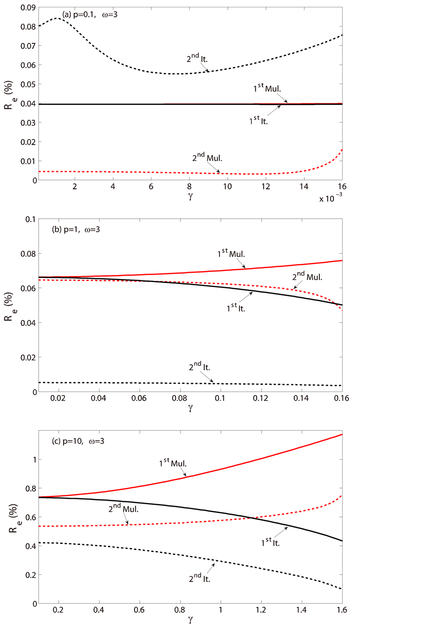
Figure 2. Global residual error (a) p = 0.1, (b) p = 1, and (c) p = 10 at ω = 3.
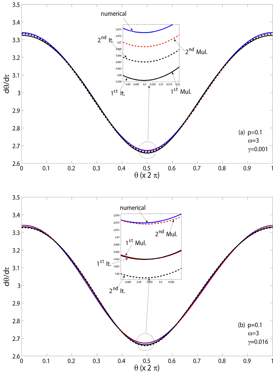
Figure 3. Phase portrait over one period (a) γ = 0.001, (b) γ = 0.016 at p = 0.1 and ω = 3.
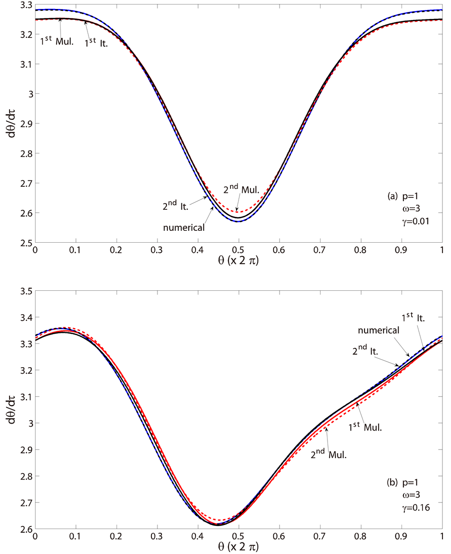
Figure 4. Phase portrait over one period (a) γ = 0.01, (b) γ = 0.16 at p = 1 and ω = 3.
ones, only the results for C1 to C8 are presented. As can be seen from Figure 6, when more iterations were performed, most of the coefficients converged quickly―within two or three iterations after being introduced. Especially for low-level excitation, i.e. p = 0.1, part of the coefficients had only small fluctuation around a certain value. In addition, for all the cases considered, the coefficients generated from three or more iterations, i.e. C5 and higher, were insignificant. Therefore, only one or two iterations are needed practically to predict the solution of period-one rotation.

Figure 5. Phase portrait over one period (a) γ = 0.1, (b) γ = 1.6 at p = 10 and ω = 3.
The lower bound of the excitation amplitude is shown in Figure 7. Three damping ratios, i.e. γ = 0.1, γ = 0.2, and γ = 0.3, were considered. The results from numerical simulation using the Dormand-Prince method (ODE45 in MATLAB©) and theoretical approximations obtained from the first and second iterations are both shown for comparison. At low frequencies, the prediction of the first iteration underestimated the lower bound, while the prediction of the second iteration slightly overestimated. However, the discrepancy diminished with the increase of the excitation frequency.
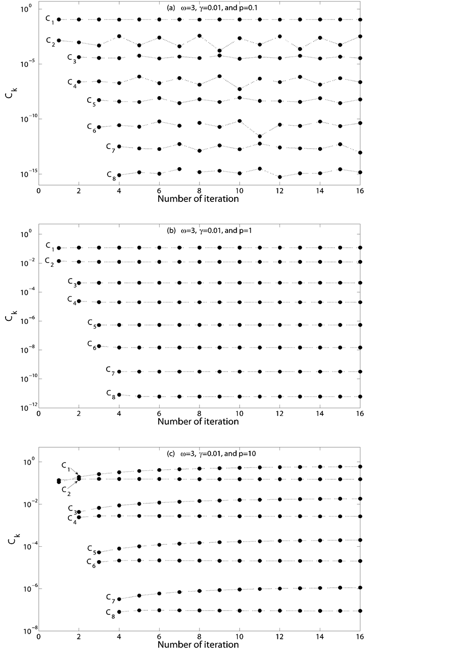
Figure 6. Convergence of coefficients Ck, k = 1, 2, ∙∙∙, 8 (a) p = 0.1, (b) p = 1, and (c) p = 10 at ω = 3 and γ = 0.01.
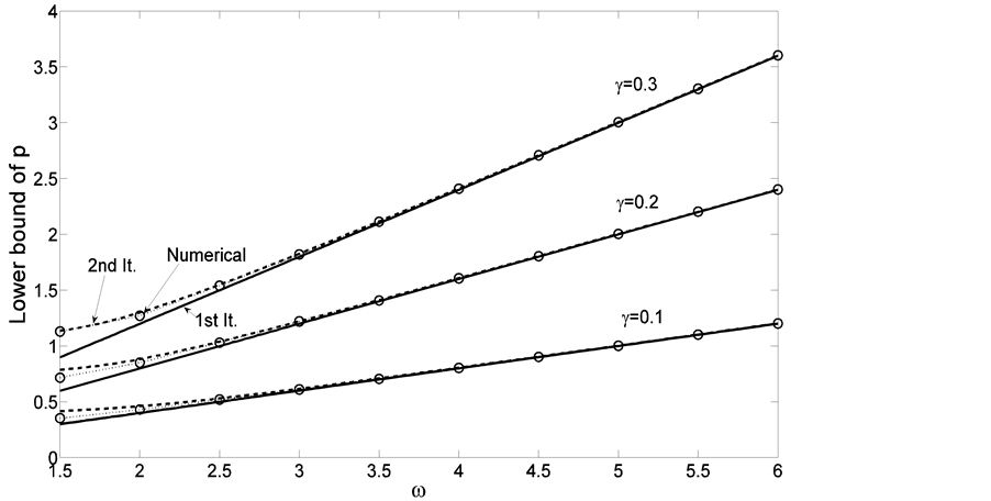
Figure 7. Lower bound of p “˗” Prediction of first iteration, “- - -” Prediction of second iteration, “…o…” Numerical simulation.
5. Concluding Remarks
In this study, period-one rotating solution of a horizontally excited pendulum was solved by the iterative harmonic balance method. The general formulas of solutions were derived. The numerical solution obtained from the Dormand-Prince method (ODE45 in MATLAB©) was used as the baseline for performance evaluation. The performance of the solutions was evaluated by two criteria, one based on the system energy error and the other based on the global residual error. The results showed that two iterations were sufficient for a reasonable accuracy. In addition, the solutions based on the multi-scale method were also shown for comparison. Under lower- level excitations, the performance of solution based on the multi-scale method was slightly better than that of the iterative method. Under higher-level excitations, however, the iterative harmonic balance method was more accurate.
Acknowledgements
This research was partially supported by National Science Foundation (Grant No. CMMI 0758632). Such generous support is greatly acknowledged.
References
- Kautz, R.L. and Macfarlane, J.C. (1986) Onset of Chaos in the rf-Biased Josephson Junction. Physical Review A, 33, 498-509. http://dx.doi.org/10.1103/PhysRevA.33.498
- Thompson, J.M.T. (1989) Chaotic Phenomena Triggering the Escape from a Potential Well. Proceedings of the Royal Society of London A, 421, 195-225. http://dx.doi.org/10.1098/rspa.1989.0009
- Bryant, P.J. and Miles, J.W. (1990) On a Periodically Forced, Weakly Damped Pendulum. Part 1: Applied Torque. The Journal of the Australian Mathematical Society. Series B. Applied Mathematics, 32, 1-22. http://dx.doi.org/10.1017/S0334270000008183
- Bryant, P.J. and Miles, J.W. (1990) On a Periodically Forced, Weakly Damped Pendulum. Part 2: Horizontal Forcing. The Journal of the Australian Mathematical Society. Series B. Applied Mathematics, 32, 23-41. http://dx.doi.org/10.1017/S0334270000008195
- Bryant, P.J. and Miles, J.W. (1990) On a Periodically Forced, Weakly Damped Pendulum. Part 3: Vertical Forcing. The Journal of the Australian Mathematical Society. Series B. Applied Mathematics, 32, 42-60. http://dx.doi.org/10.1017/S0334270000008201
- Koch, B.P. and Leven, R.W. (1985) Subharmonic and Homoclinic Bifurcations in a Parametrically Forced Pendulum. Physica, 16D, 1-13.
- Leven, R.W., Pompe, B., Wilke, C. and Koch, B.P. (1985) Experiments on Periodic and Chaotic Motions of Aparametrically Forced Pendulum. Physica, 16D, 371-384.
- Clifford, M.J. and Bishop, S.R. (1995) Rotating Periodic Orbits of the Parametrically Excited Pendulum. Physics Letters A, 201, 191-196. http://dx.doi.org/10.1016/0375-9601(95)00255-2
- Garira, W. and Bishop, S.R. (2003) Rotating Solutions of the Parametrically Excited Pendulum. Journal of Sound and Vibration, 263, 233-239. http://dx.doi.org/10.1016/S0022-460X(02)01435-9
- Ma, T.W. and Zhang, H. (2012) Enhancing Mechanical Energy Harvesting with Dynamics Escaped from Potential Well. Applied Physics Letters, 100, Article ID: 114107. http://dx.doi.org/10.1063/1.3694272
- Xu, X. and Wiercigroch, M. (2007) Approximate Analytical Solutions for Oscillatory and Rotational Motion of Aparametric Pendulum. Nonlinear Dynamics, 47, 311-320. http://dx.doi.org/10.1007/s11071-006-9074-4
- Lenci, S., Pavlovskaia, E., Rega, G. and Wiercigroch, M. (2008) Rotating Solutions and Stability of Parametric Pendulum by Perturbation Method. Journal of Sound and Vibration, 310, 243-259. http://dx.doi.org/10.1016/j.jsv.2007.07.069
- Zhang, H. and Ma, T.W. (2012) Iterative Harmonic Balance for Period-One Rotating Solution of Parametric Pendulum. Nonlinear Dynamics, 70, 2433-2444. http://dx.doi.org/10.1007/s11071-012-0631-8
- Pavlovskaia, E., Horton, B., Wiercigroch, M., Lenci, S. and Rega, G. (2012) Approximate Rotational Solutions of Pendulum under Combined Vertical and Horizontal Excitation. International Journal of Bifurcation and Chaos, 22, 1250100-1250113.
Appendix
nth Iteration (n > 3)
In the nth iteration, the modified governing equation is
 . (22)
where  is obtained from the (n − 1)th iteration.
The solution of Equation (22) can be obtained as
 . (23)
where
 . (24)
and
 (25)
(25)
in which
 (26)
(26)
and
 (27)
(27)
As  is bounded in [−1, 1], the necessary condition for solution to exist is
 . (28)