World Journal of Mechanics
Vol.2 No.1(2012), Article ID:17679,8 pages DOI:10.4236/wjm.2012.21001
Modulation Equations for Roll Waves on Vertically Falling Films of a Power-Law Fluid
1Laboratoire de Mecanique de Lille, Villeneuve d’Ascq, France
2Lavrentyev Institute of Hydrodynamics, Novosibirsk State University, Novosibirsk, Russia
Email: abdelaziz.boudlal@univ-lille1.fr, liapid@hydro.nsc.ru
Received November 20, 2011; revised December 20, 2011; accepted December 30, 2011
Keywords: Power-Law Fluid; Thin Film Flow; Vertical Wall; Modulation Equations; Nonlinear Stability; Roll Wave
ABSTRACT
Waves of finite amplitude on a thin layer of non-Newtonian fluid modelled as a power-law fluid are considered. In the long wave approximation, the system of equations taking into account the viscous and nonlinear effects has the hyperbolic type. For the two-parameter family of periodic waves in the film flow on a vertical wall the modulation equations for nonlinear wave trains are derived and investigated. The stability criterium for roll waves based on the hyperbolicity of the modulation equations is suggested. It is shown that the evolution of stable roll waves can be described by self-similar solutions of the modulation equations.
1. Introduction
Mud flows are frequently encountered in mountainous regions, especially after torrential rains, and often exhibit a series of breaking waves (roll waves). These type of waves can also be observed as an event following volcano eruptions. A report on roll waves can be found in extensive references quoted by Ng & Mei [1]. The roll waves which occur in inclined open channels are important in drainage problems and have received an extensive treatement in turbulent regime by Jefffreys [2], Dressler [3], Boudlal & Liapidevskii [4], among others, and for a laminar sheet flow by considering the flow with quadratic distribution of velocity profile (Alekseenko & Nakoryakov [5]; Buchin & Shaposhnikova [6]; Julien & Hartley [7]; Boudlal & Liapidevski [8]).
The discontinuous waves play an important role in engineering and geophysical processes. Roll waves consist of a periodic pattern of bores separated by continuous profiles of free boundary. The transition from uniform flow to intermittent flow regime is usually tackled by resorting to stability theory. When it is perturbed, a steady flow becomes unstable, if certain criteria are satisfied, and evolves towards wave breaking. Dressler has been the first, who gave the analytical solution for such waves in open channel flows. Based on long wave approximation, Dressler’s theory of roll waves was extended in [1] to a shallow layer of fluid mud, which has been modelled as a power law fluid. It has been shown, particularly, that if the fluid is highly non-Newtonian, very long waves may still exist even if the corresponding uniform flow is stable to infinitesimal perturbations.
The aim of the paper is to give a nonlinear study on stability of permanent roll waves on a shear thinning fluid in the frame of one-dimensional, unsteady, gradually varied, laminar mud flow with the shear stress being evaluated in a conventional manner. Starting from long waves equations averaged over the normal to the bed [1], the standard procedure of roll wave construction is used by matching continuous solutions of shallow water equations through stable hydraulic jumps. As the amplitude and the phase velocity of waves are slowly varying during their propagation and as these variations give rise to instability, the problem of stability is solved by deriving modulation equations for wave series. The stability criterion is formulated in terms of hyperbolicity of modulation equations that need the calculation of averaged quantities.
All results presented herein can be regarded as a generalization to a power law mud fluid in laminar flow regime of non linear stability method alredy applied to Newtonian turbulent flows in open channels (Boudlal & Liapidevskii [9]).
2. Governing Equations
Consider two-dimensional film flows of a non-Newtonian liquid on a vertical wall. The coordinate system  is defined as follows: the
  axis is directed vertically down and
  axis is horizontal and directed outward of the liquid layer. The longitudinal velocity component is denoted by
  The boundary layer approximation is assumed to be valid, with a power-law shear stress relation for laminar flows taken in the form
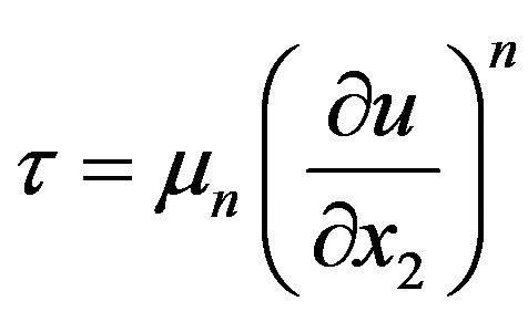 (2.1)
(2.1)
Here  is the viscosity coefficient of dimension
 and
and  is the flow index
 . The case n = 1 corresponds to the Newtonian fluid and
  is the ordinary dynamic viscosity [1]. By assuming the following form of the velocity profile in the film flow
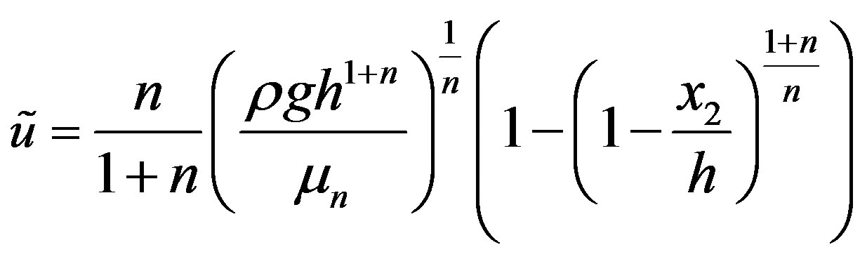 , (2.2)
the governing equations, which consist of the mass and momentum conservation equations averaged in the ordinate direction, are reduced to the system [1].
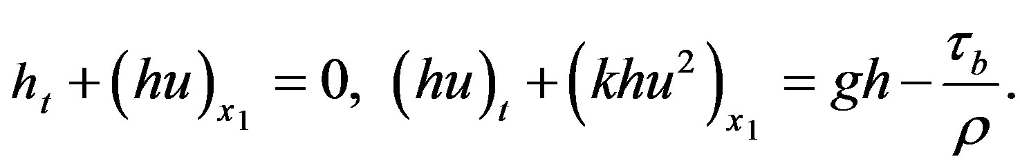 (2.3)
(2.3)
Here h is the layer thickness,  is the depth-averaged velocity,
 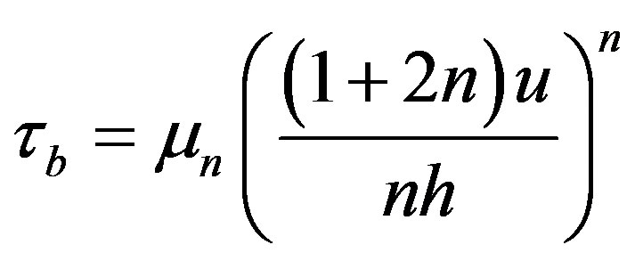 is the bottom stress, g is the gravity acceleration,
 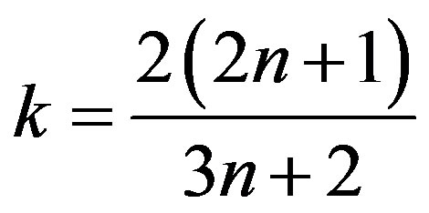 is the momentum flux factor. For a shear-thinning fluid, which will be considered bellow, we have
  and, consequently,
 .
.
In dimensionless variables introduced in [1]; namely,
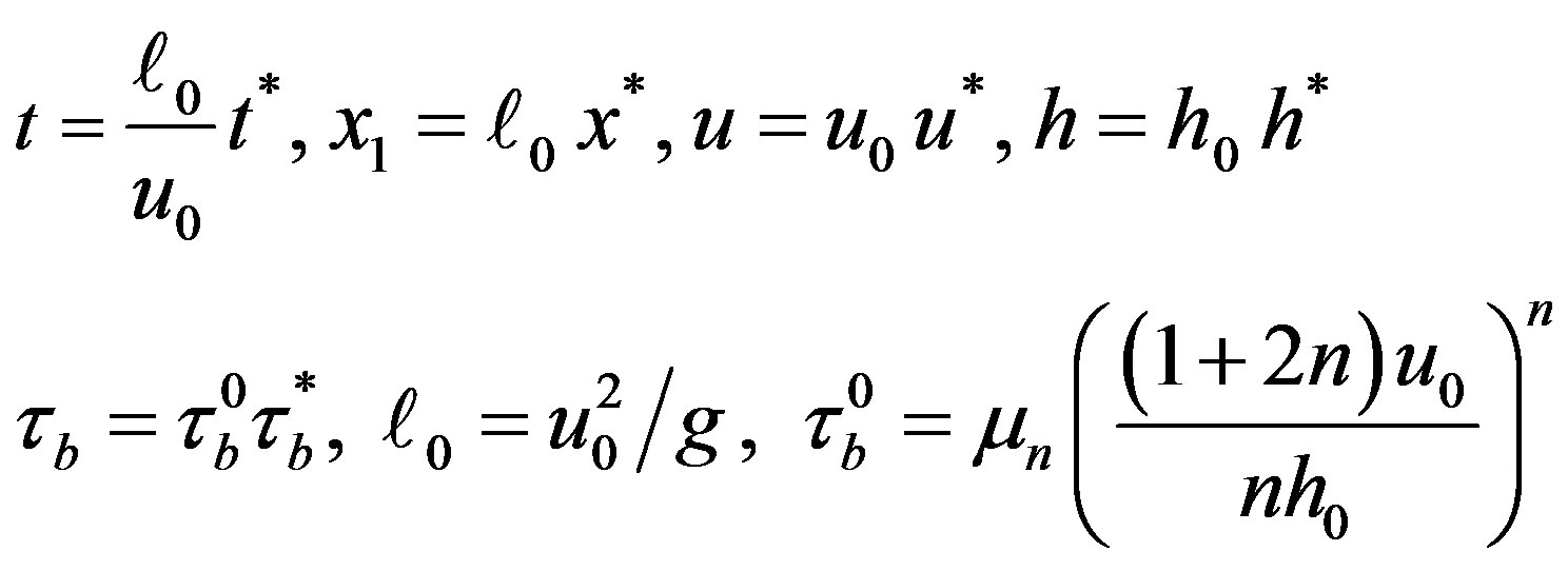 (2.4)
(2.4)
Equation (2.3) take the form (asterisks are omitted)
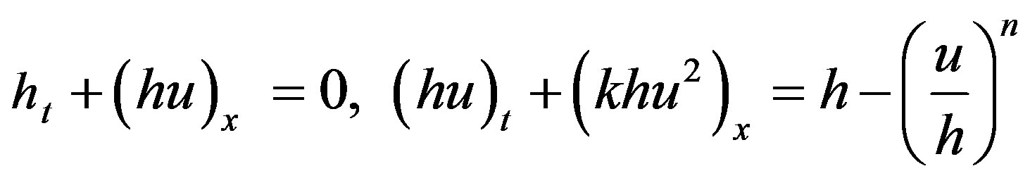 (2.5)
(2.5)
Here the reference depth  and the reference velocity
  are expressed through the given flow rate
  and the viscosity
  as follows:
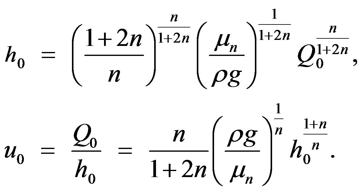 (2.6)
(2.6)
Note that Equation (2.5) are hyperbolic with the characteristics
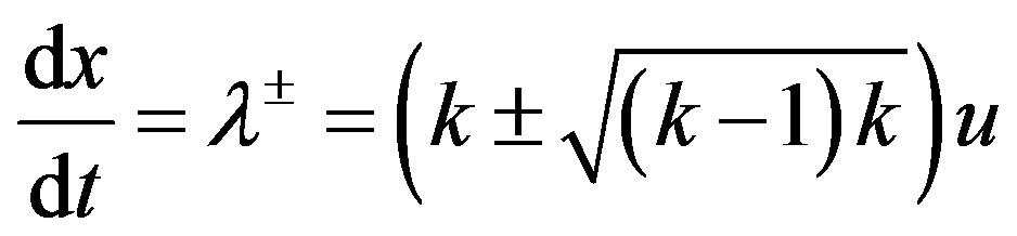 . (2.7)
It is shown by linear analysis in [1] that any steady-state solution of (2.5)
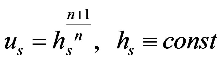
is unstable. The instability of the uniform steady-state flow also can be easily checked by the Whitham method [9]. The flow is unstable if the velocity of the kinematic wave  exceeds the velocity of long waves in (2.5), i.e.
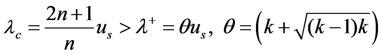 . (2.8)
It is clear that (2.8) is satisfied for , since
 and
and .
.
3. Roll Waves
Analogously to unstable flow regimes in open channel flows, the roll waves or periodic discontinuous solutions, have been constructed for (2.5) [1]. In this section we give the short description of roll waves in the form suitable for the purposes of the paper.
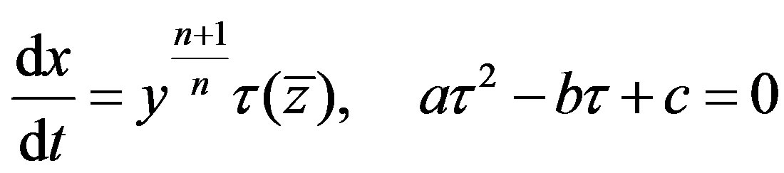
Consider the travelling waves propagating with a constant velocity . Introducing the variable
  and assuming the flow being steady in the coordinate system moving with the velocity
 , Equation (2.5) are reduced to the ODE
 , (3.1)
where 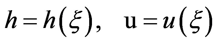 and
and
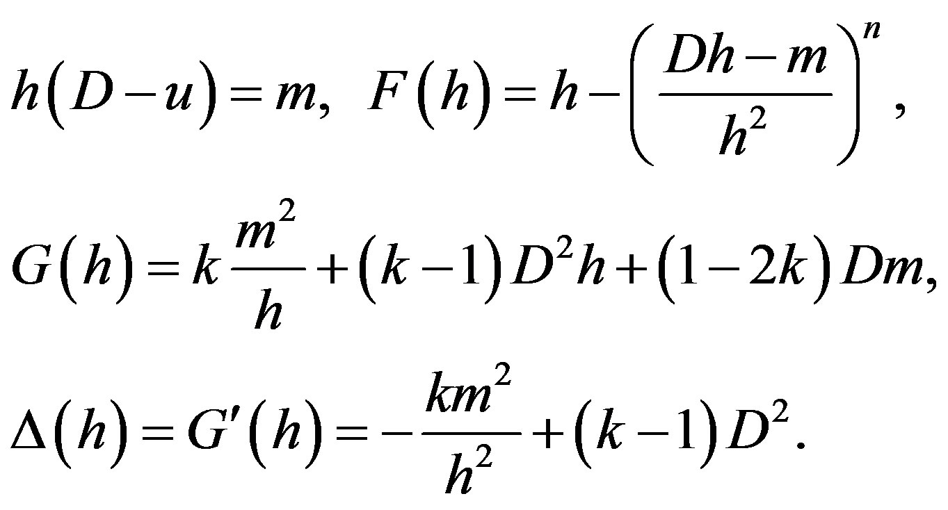 (3.2)
(3.2)
Let y and  be the critical depth and the critical velocity with
  It follows from (3.1) that the necessary condition of roll wave existence is
 (3.3)
(3.3)
In view of (3.2) we have
 . (3.4)
Note that
 (3.5)
(3.5)
and, consequently,  at the critical depth.
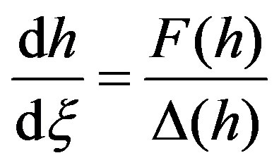
Let  be fixed and
 . Equations (3.1)-(3.2) take the form
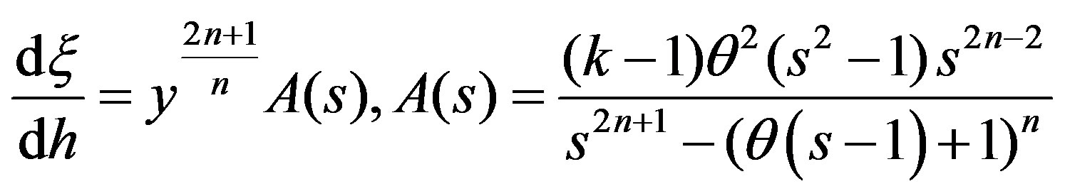 . (3.6)
To find the function  in (3.6), the following identity is used:
 .
.
Furthermore, the function  can be represented as follows
 (3.7)
(3.7)
where , and
, and  is a root of the equation
  at the interval
 . The continuous function
is positive for . It means that the function
  vanishes only at two points
  and
and  for
for  [1]. Therefore,
  for
for  and
and
 .
.
Now we can construct the two-parameter family of roll waves as follows: for given  and
and  we put
 ,
,  ,
, . Note that
  and
and  are the conjugate depths, since the Rankine-Hugoniot conditions for discontinuous solutions of (2.5), which are reduced to the relation
 or
or
 ,(3.8)
are fulfilled. The stability condition for shocks satisfying (3.8) takes the form (Rozhdestvenskii and Janenko [10])
 or
or
 (3.9)
(3.9)
Thus the admissible values of the governing parameters , for which a roll wave exists, belong to the domain

For , a roll wave consists of the smooth part defined by the monotonous solution
  of (3.6) at the interval
  and of the jump with the conjugate depths
  and
and 
4. Modulation Equations
It is shown in the previous section that analogously to the roll waves in open channel flows governed by the classic shallow water theory (Whitham [10]), the periodic travelling waves (roll waves) in film flow of a non-Newtonian fluid can be represented by the two-parameter family of discontinuous solutions of (2.5). We chose  and
and  as such parameters. The problem on nonlinear stability of periodic wave trains with slowly varying values
  and
and  can be solved by analysis of hyperbolicity of the modulation equations for roll waves (Boudlal and Liapidevskii, [11]). After averaging (2.5) over the fixed length scale, which is large enough compared with the length of roll waves, we have the following modulation equations:
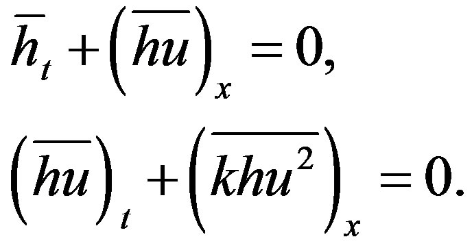 (4.1)
(4.1)
All averaged quantities can be expressed as functions of  and
and  as follows :
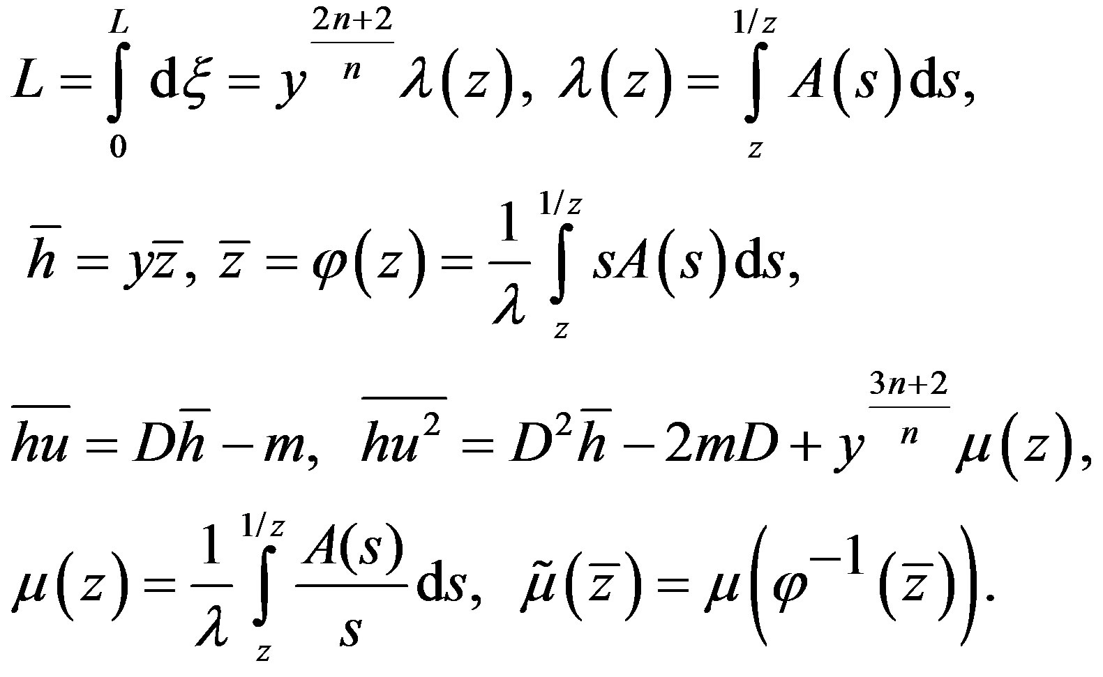 (4.2)
(4.2)
Here we have used (3.1)-(3.2), (3.8) for periodic roll waves defined by parameters  and
and .
.
In view of (4.2) and (3.4) the modulation equations take the form
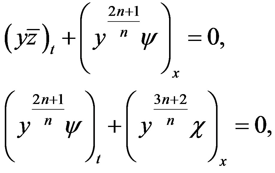 (4.3)
(4.3)
where
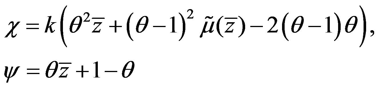 (4.4)
(4.4)
The nonstationary evolution of the governing parameters  for a periodic wave train is described by Equation (4.3). We say the roll waves are stable if the modulation Equation (4.3) for corresponding values
  are hyperbolic. Considering
  and
and  as new dependent variables instead of
  and
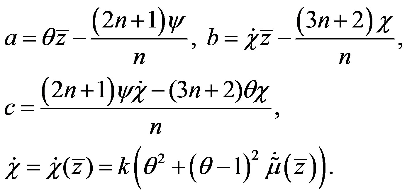
and , we can find the characteristics of (4.3) from the quadratic equation
 (4.5)
(4.5)
where
 (4.6)
(4.6)
Here “·” denotes the differentiation on  and
and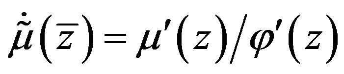 .
.
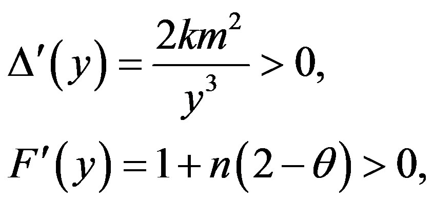
Equation (4.3) are hyperbolic for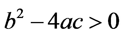 . It means that the hyperbolicity domain depends only on the variable
  or
or  Note that
  for
for . It can be shown by numerical calculations that the hyperbolicity interval is rather narrow and it lies in vicinity of
 . For n = 1
  the values of
  corresponding to the hyperbolicity domain belong to the interval
  with
with  Therefore, the boundary of the hyperbolicity domain can be found effectively by the following approximation of the function
  for long waves
 (4.7)
(4.7)
Approximate values of characteristics are given by (4.5)-(4.6) with  instead of
  and
and  instead of
 . In this case the modulation equations simplify considerably since the functions
  and
and  are linear on
 :
:
 (4.8)
(4.8)
The dependence  for Equations (4.3), (4.8) with n = 1 is shown in Figure 1 for real roots of (4.5) (
 ). Note that the corresponding graphs for (4.3), (4.4) and the approximate system (4.3), (4.8) practically concide, so we can use the latter system for the analysis of nonlinear stability of roll waves in the flows governed by (2.5). It follows from Figure 1 that the hyperbolicity interval
  for (4.3), (4.8) lies inside of the admissible interval of roll wave existence
 . It means that short roll waves
  and very long roll waves
  are unstable.
The simple centered waves, i.e. the self-similar solutions of (4.3) depending on the variable , can be found analytically. Equations (4.3), (4.8) for simple
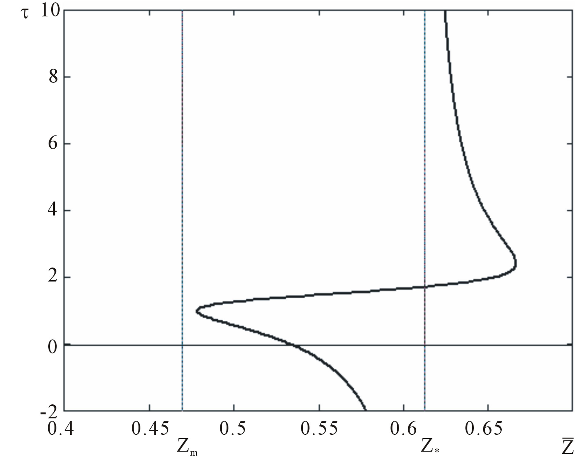
Figure 1. Dependence  for (4.3), (4.8).
waves take the form
 (4.9)
(4.9)
A solution of (4.9) can be represented in the form
 (4.10)
Here  is a solution of (4.3) for the corresponding family of characteristics. The solution (4.10) can be applied to explain some specific features of roll wave dynamics considered below.
5. Roll Wave Dynamics
In this section we compare the numerical calculations performed for the model derived by Meza and Balakotaiah (2008) for vertically falling films of Newtonian fluid with numerical solutions of (2.3) for n = 1. Both models are derived for moderate Reynolds numbers of flow, but in contrast to the former model, the surface tension in Equation (2.3) is ignored. Let us rescale (2.3) slightly according to (Meza and Balakotaiah, 2008). For that we introduce the Reynolds number  and the Weber number
  as follows
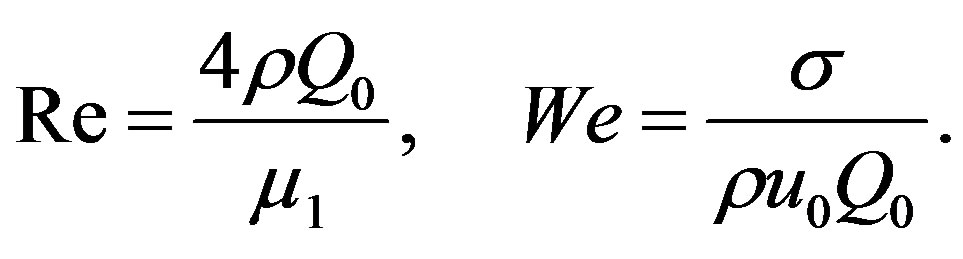
Here  is the surface tension. Consider two models of film flows on a vertical wall depending on
  and
and  explicitly. The first one is the Shkadov model [12], which with the dependent variables
  and
and 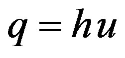 takes the form
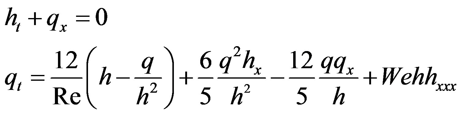 (5.1)
(5.1)
It is clear that for  and
and . Equations (2.5) are equivalent to (5.1) and the systems can be transformed to each other by dilatation of independent variables. The momentum equation derived by Meza and Balakotaiah [13] gives the more accurate dispersion relations comparing with the Shkadov model as it has reported in their paper:
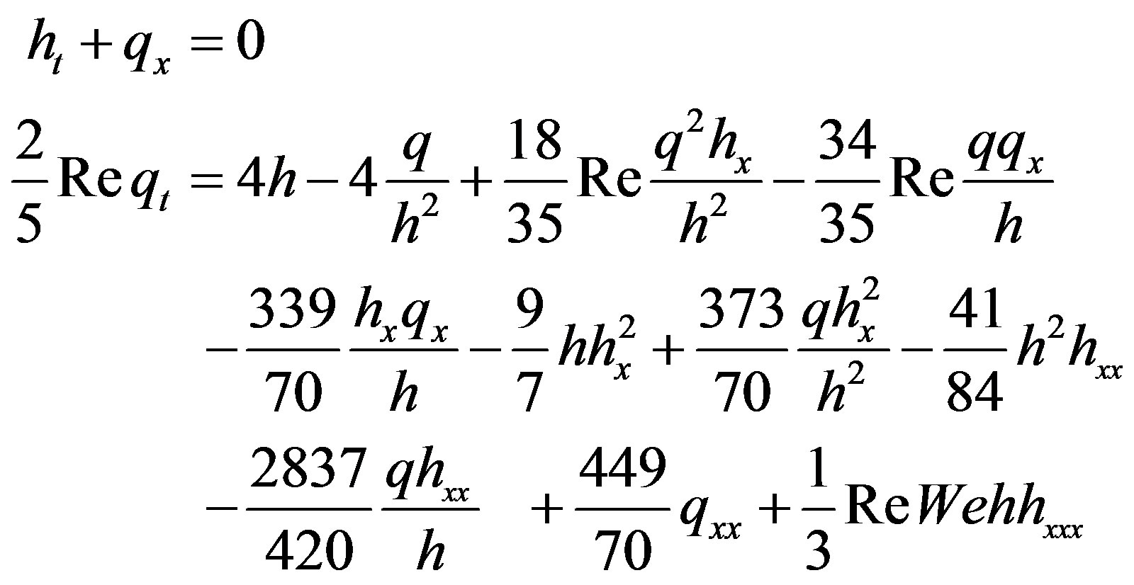 (5.2)
(5.2)
We will compare below numerical solutions of the model (5.2) presented in [13] with the corresponding numerical solutions of the hyperbolic model (5.1) with . It will be shown that despite of the difference in the shape of individual roll waves for the models with and without surface tension, the evolution of nonlinear periodic wave trains generated by monochromatic initial perturbations is very alike for both models. Note that Equations (5.1) and (5.2) are written in dimensionless variables. The characteristics of (5.1) with
  coincide with (2.7) and are positive. Therefore, to find a solution of (5.1) in the domain
 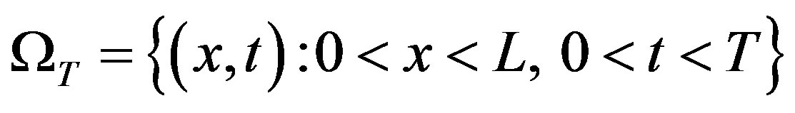 , we must put the values of
  at the boundaries
  and
and . The corresponding data are taken from (Meza and Balakotaiah, 2008) for the cases considered in their paper, namely:
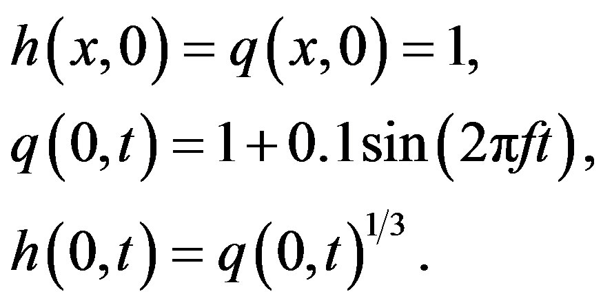 (5.3)
(5.3)
We restrict our attention to the case 1 in [13] with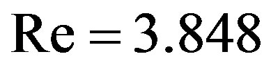 . The Weber number for (5.2) is finite (
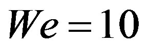 ) and it vanishes for (5.1). The values of the dimensionless frequency
  are varied to demonstrate its influence on roll wave dynamics.
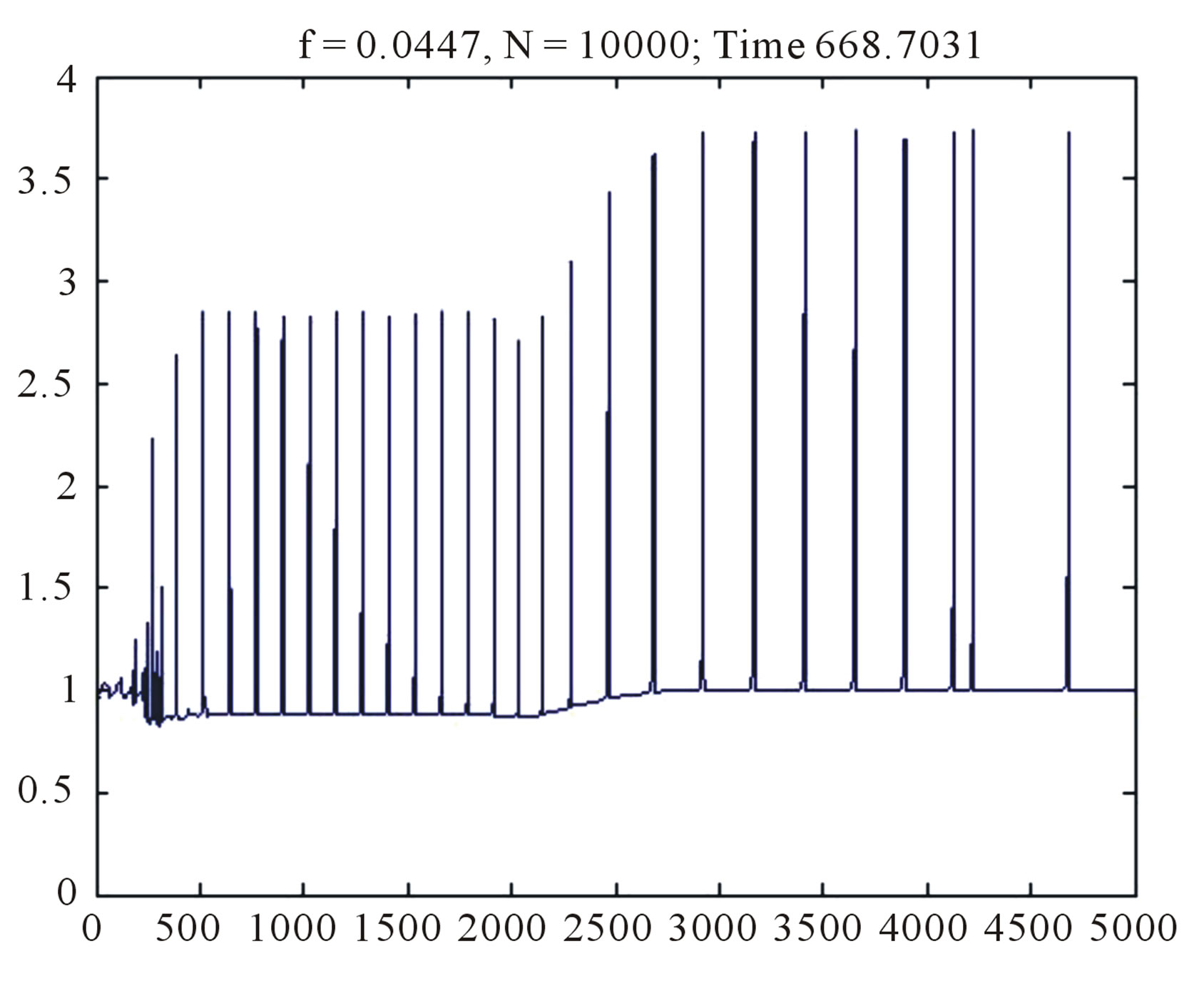
Numerical calculations using a variant of the Godunov standard scheme illustrate the development of roll waves on the free surface of a thin film flowing on a vertical wall in the frame of the hyperbolic model (5.1). In Figures 2-4 the perturbations of free surface of the liquid layer calculated by (5.1) are comparing with correspond-
 (a)
(a)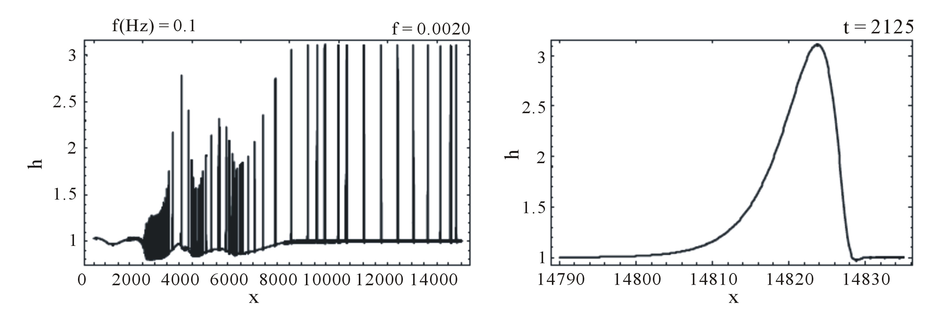 (b)
(b)
Figure 2. Wave profile in the forced film flow of the Newtonian fluid (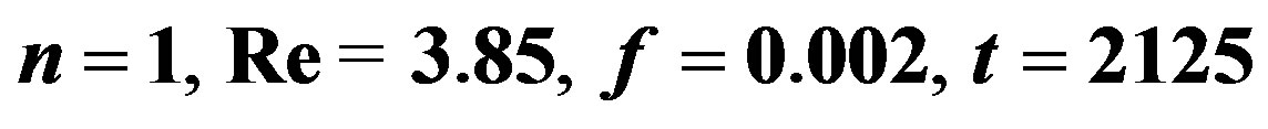 ): (a) Equation (5.1), We = 0; (b) Equation (5.2), We = 10.
 (a)
(a)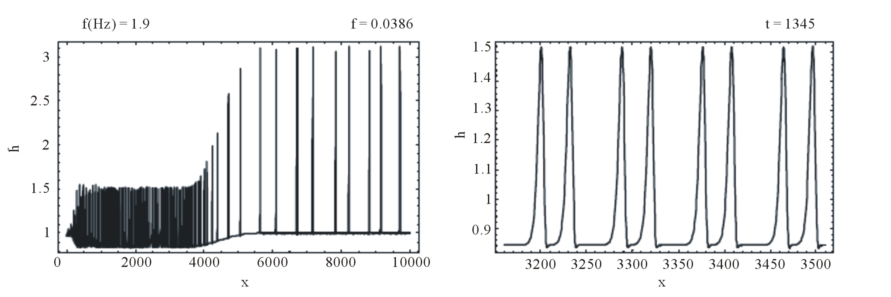 (b)
(b)
Figure 3. Wave profile in the forced film flow of the Newtonian fluid ( ): (a) Equation (5.1), We = 0; (b) Equation (5.2), We = 10.
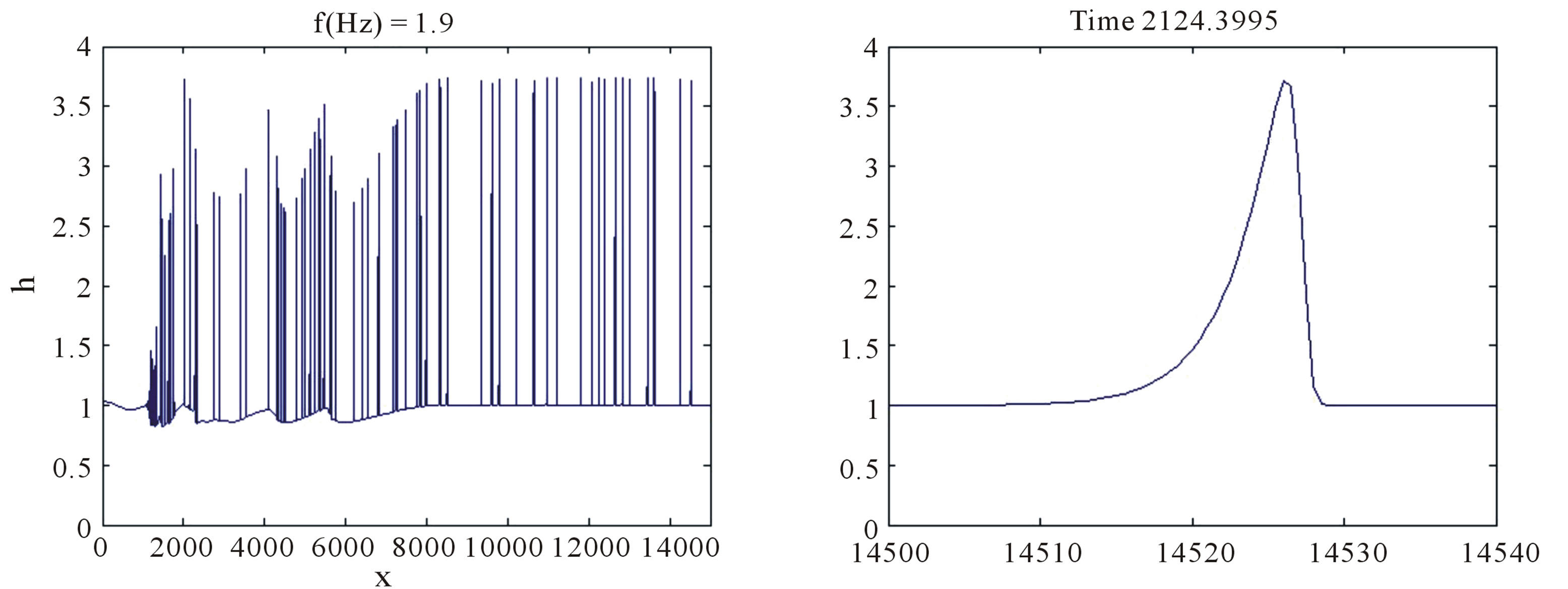
ing calculations from [13], at given time. In both cases small perturbations, which amplitudes do not exceed a small fraction of the depth of the initial steady-state flow, are developing into roll waves of finite amplitude. Note that the waves stop to grow after they reach some critical value of amplitude. The interesting feature of roll wave evolution is the transition from “saturated” waves to very long waves (“tsunami” waves according [11]). Such transition is most pronounced in Figure 4. It is seen from Figures 4(a)-(c) that the length of the transition zone is increasing with time linearly. The analysis of the nonstationary evolution of roll wave packets is the subject of future investigations. Here we just give an idea how the self-similar solutions (4.10) can be applied to describe the transition “0” - “1” shown in Figures 4(a)-(c). First of all, for given frequency  of the monochromatic wave packet “0”, the governing parameters
  are uniquelly determined by (3.4), (4.2), (4.7). Furthermore, in virtue of (4.10) the left boundary
  of the centered simple wave is known. The right boundary of the simple wave is calculated using (4.10) and the additional condition for “tsunami” waves:
 .
.
This algorithm gives the reasonable values for the boundaries of the states “0” and “1” in numerical calculations of the nonstationary problem of roll wave evolution. Therefore, the transition “0” - “1” in Figures 4(a)- (c) can be described by the centered simple wave of (4.9) moving on the left  and the roll waves shown in Figure 4 are stable, since the governed parameters
  in a simple wave always belong to the hyperbolicity domain of the modulation equations
6. Conclusion
We have investigated the roll wave generation on vertically falling films by the nonlinear hyperbolic model (2.3), in which the viscous effects are taken into account by assuming that the velocity profile of an exact steady-state solution of the two-dimensional problem can be used also in the one-dimensional wavy flows. The model is based on the first order long-wave approximation of non-Newtonian fluid flows, which shear rate is modeled by a power law [1]. The capillarity effects are ignored to reveal the interplay between nonlinear and viscous terms in the governing equations. It is shown that
 (a)
(a)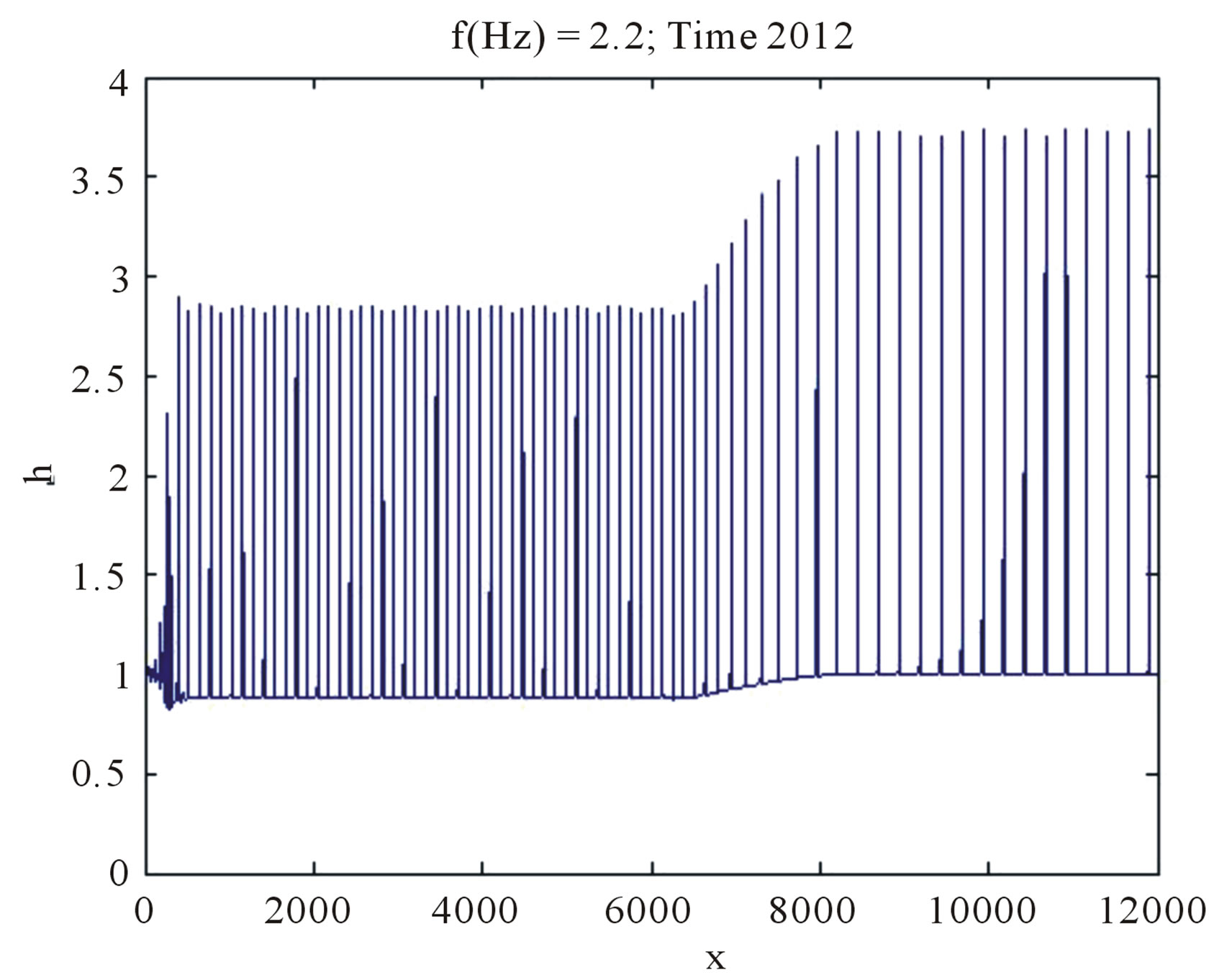 (b)
(b)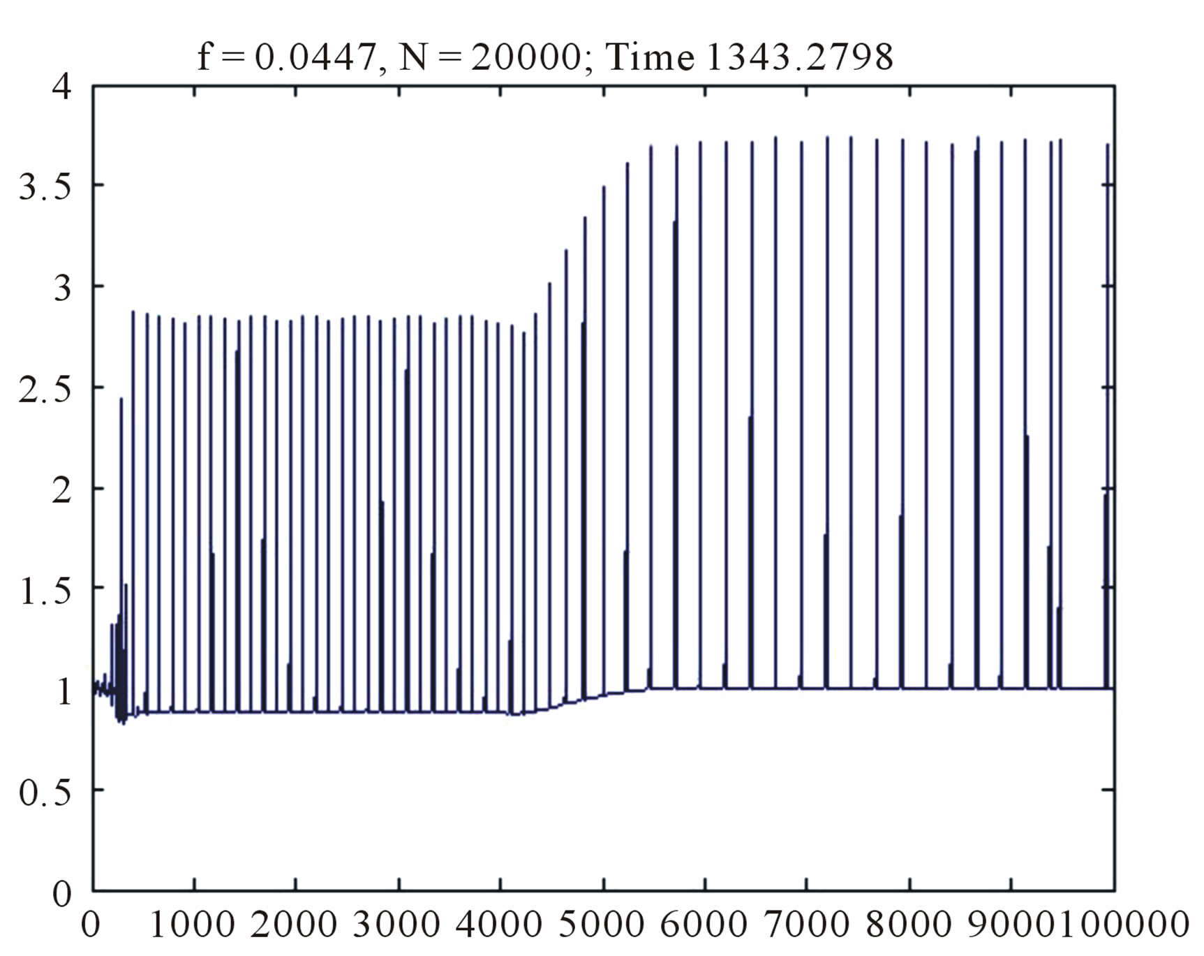 (c)
(c)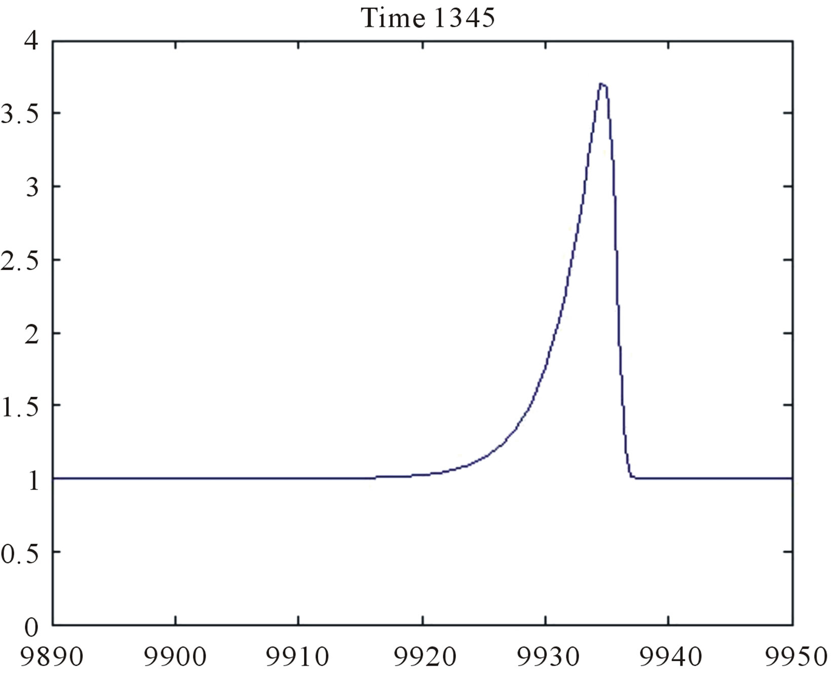 (d)
(d)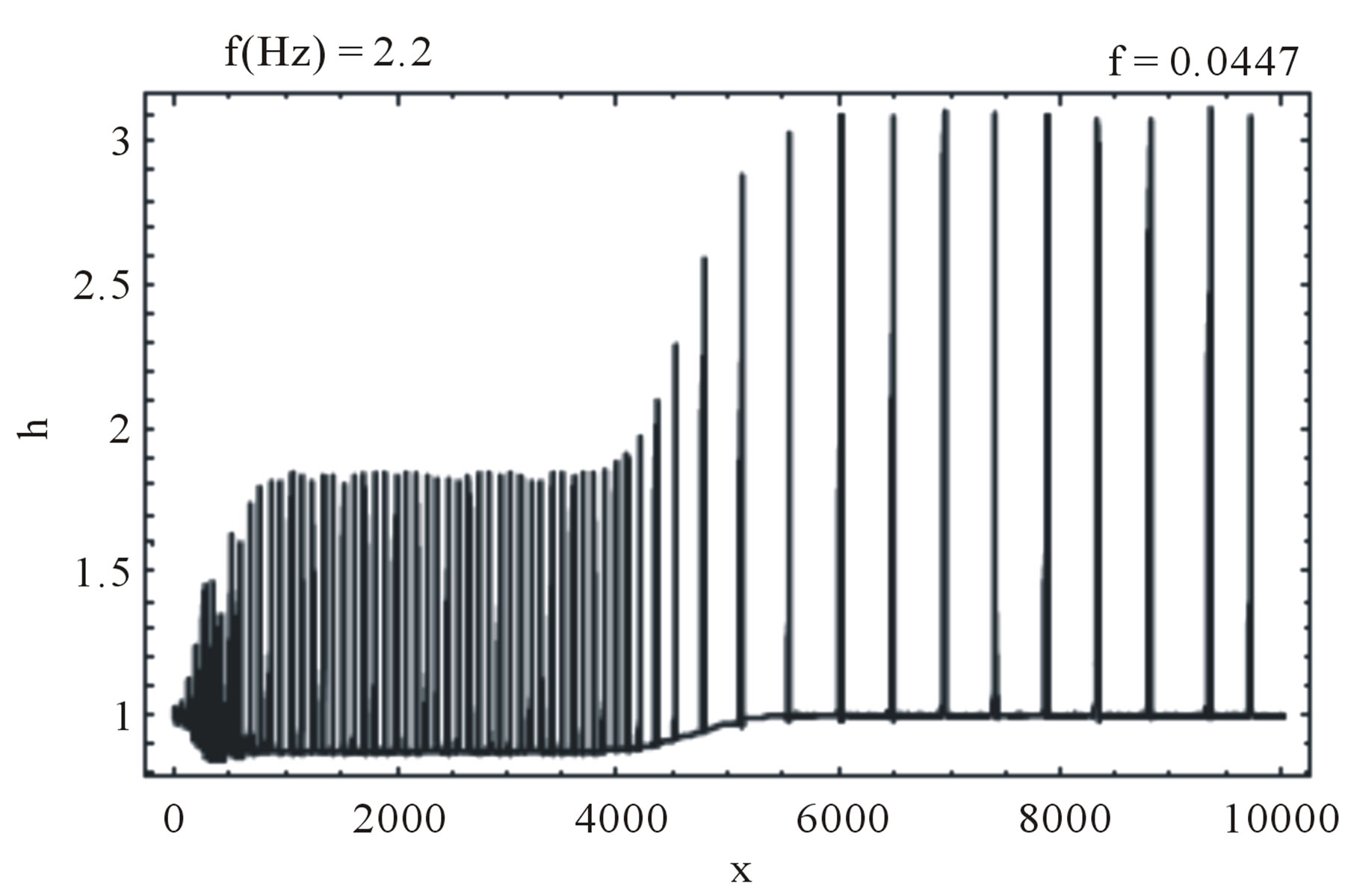 (e)
(e)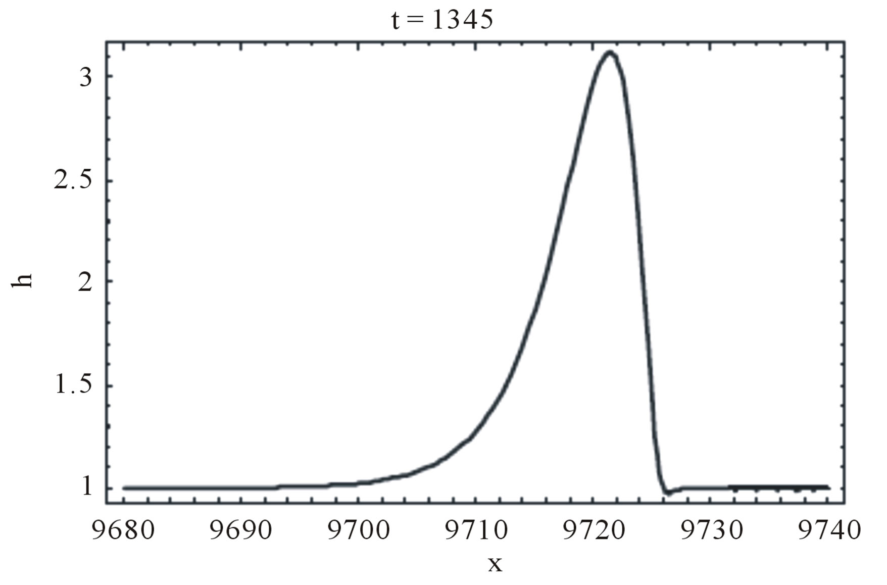 (f)
(f)
Figure 4. Wave profile in the forced film flow of the Newtonian fluid ( ): (a)-(d) Equation (5.1), We = 0; (e)-(f) Equation (5.2), We = 10; (a)
 ; (b)
; (b) ; (c)-(f)
 .
.
the periodic discontinuous solutions of (2.3) (roll waves) can be described by two parameters analogously to the roll waves in open channel flows. Moreover, the nonlinear stability of finite amplitude roll waves can be expressed in the terms of the hyperbolicity of modulation Equations (4.3) for the governing parameters of roll waves. Comparison of numerical calculations of roll wave evolution for the models with and without surface tension effects reveal that in spite of the difference in the individual wave shapes the behavior of roll wave packets is very alike for the models. In particular, the transition from “saturated” to “tsunami” waves described in [13] can be described by a simple wave of the modulation Equations (4.3).
7. Acknowledgements
The work was supported by the Russian Foundation for Basic Research (Grant No. 10-01-00338) and by the Program for support of leading scientific schools of the Russian Federation (Grant No. NSh-6706.2012.1).
REFERENCES
- C. O. Ng and C. C. Mei, “Roll Waves on Shallow Layer of Mud Modelled as a Power-Law Fluid,” Journal of Fluid Mechanics, Vol. 263, 1994, pp. 151-1834.
- T. Jeffreys, “The Flow of Water in Inclined Channel of Rectangular Section,” Philosophical Magazine, Vol. 49, No. 6, 1925, pp. 793-807.
- F. Dressler, “Mathematical Solution of the Problem of Roll Waves in Inclined Open Channels,” Communications on Pure and Applied Mathematics, Vol. 2, No. 2-3, 1949, pp. 149-194. doi:10.1002/cpa.3160020203
- A. Boudlal and V. Yu. Liapidevskii “Stability of Roll Waves in Open Channels,” Comptes Rendus Mécanique, Vol. 330, No. 4, 2002, pp. 209-295. doi:10.1016/S1631-0721(02)01461-4
- S. V. Alekseenko, V. E. Nakoryakov and B. G. Pokusaev, “Wave Flow in Liquid Films,” Begell House, New York, 1994.
- V. A. Buchin and G. A. Shaposhnikova, “Flow of Shallow Water with a Periodic System of Jumps over a Vertical Surface,” Doklady Physics, Vol. 54, No. 5, 2009, pp. 248-251. doi:10.1134/S1028335809050073
- P. Y. Julien and D. M. Hartley, “Formation of Roll Waves in Laminar Sheet Flow,” Journal of Hydraulic Research, Vol. 24, No. 1, 1986, pp. 5-17. doi:10.1080/00221688609499329
- A. Boudlal and V. Yu. Liapidevskii, “Stability of Roll Waves on a Vertical Wall,” International Conference “Fluxes and Structures in Fluids: Physics of Geospheres”, Moscow, 2010, pp. 48-53.
- A. Boudlal and V. Yu. Liapidevskii, “Stability of Regular Roll Waves,” Computation Technologies, Vol. 10, No. 2, 2004, pp. 3-14.
- B. L. Rozhdestvenskii and N. N. Janenko, “Systems of Quasilinear Equations and Their Application to Gaz Dynamics,” American Mathematical Society Translations: Series 2, Vol. 55, 1983.
- G. B. Whitham, “Linear and Nonlinear Waves,” John Wiley and Sons, New York, 1974.
- V. Ya. Shkadov, “Theory of Wave Flows of a Thin Layer of a Viscous Liquid,” Izvestiya Akademii Nauk SSSR Mekhanika Zhidkosti I Gaza, Vol. 2, 1968, pp. 20-25.
- C. E. Mesa and V. Balakotaiah, “Modelling and Experimental Studies of Large Amplitude Waves on Vertically Falling Films,” Chemical Engineering Science, Vol. 63, No. 19, 2008, pp. 4704-4734. doi:10.1016/j.ces.2007.12.030