World Journal of Mechanics
Vol. 1 No. 3 (2011) , Article ID: 5769 , 7 pages DOI:10.4236/wjm.2011.13010
3-Point Bending of Bars and Rods Made of Materials Obeying a Ramberg-Osgood Criterion
CEIT and Tecnun (University of Navarra) Paseo Manuel Lardizábal, San Sebastián, Spain
E-mail: ameizoso@ceit.es
Received March 18, 2011; revised April 19, 2011; accepted April 29, 2011
Keywords: Bending, Non-Linear, Ramberg-Oswood
ABSTRACT
Equations are derived for the non-linear bending of cantilever and 3-point bending of beams (with a non uniform moment distribution along its length) made of materials described according to Ramberg-Osgood behaviour (including and elastic and a plastic term with a hardening exponent). Moment for plastic collapse is also computed.
1. Introduction
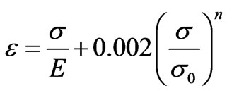
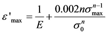
In a previous paper the non-linear bending of beams with a simple Hollomon material behaviour was obtained [1,2]. With this very simple material behaviour, it is possible to obtain analytic solutions. A more realistic material will be studied in this paper, including two terms for the deformation: elastic and plastic. The material behaviour follows a Ramberg-Osgood [3] law:
 (1)
(1)
e is the strain, s represents the stress,  is the yield stress (that corresponding to a plastic strain of 0.2%). E, the modulus of elasticity (Young’s modulus) and n, the hardening exponent, are material constants. The first term usually represents the elastic strain and the second, the plastic part of the deformation. That is the usual case for most ductile metals in which unloads result in a straight line parallel to the elastic load [4]. But it may be thought as an elastic non-linear material, and then both terms, in Equation (1) are elastic; loading and unloading follow the same trace. As far as no unloading is produced (for example, using a proportional loading) no difference will be observed between both cases: elasto-plastic and non-linear elastic.
Figure 1 shows three materials with the same Young’s modulus and yield stress but different hardening exponents. These curves are plotted to different maximum strains that will be explained later. Although it is not explicit in Equation (1), the material behaviour will be assumed symmetric i.e. identical in tension and compression (most metals behave symmetrically, and—as a particular case of—all isotropic materials, which behave identically also in all directions).
1.1. Plastic Hinge
Plastic collapse will take place whenever the strain is localized and not uniformly distributed. Considère’s criterion [5] is used and sketched in Figure 2. That is the reason why the stresses versus strain plots, in Figure 1, are limited to different maximum strains, for the different hardening exponent. From Figure 1 it is clear that plastic instability take place for large plastic strains (for the exponent being considered). If the elastic contribution is neglected, the maximum uniform strain is limited to 1/n.
1.2. Non-Linear Bending
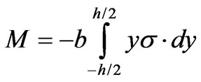
For a given bending moment, M, the stresses in the longitudinal direction, s, distribute in the section replicating the stress versus strain plots (shown in Figure 1). Bending moment is
 (2)
(2)
Or, because the identical material behaviour assumed for tension and compression
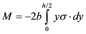 (3)
(3)
For a non-linear material, it is still valid to assume that
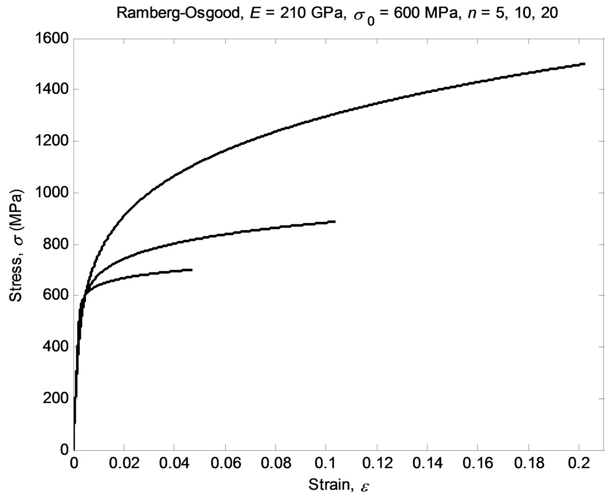
Figure 1. Stress versus strain plot for three materials behaving according to Ramberg-Osgood, Equation (1).
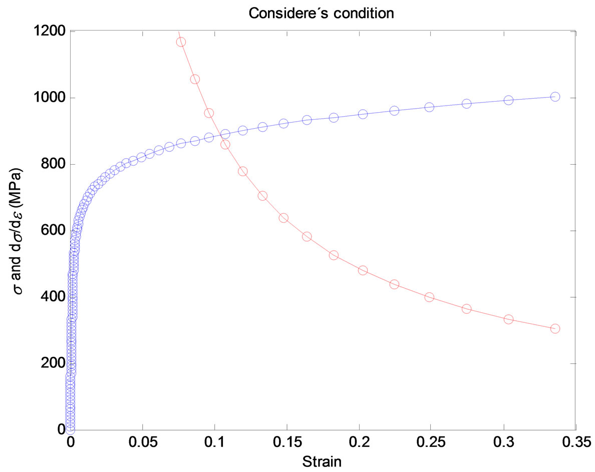
Figure 2. Considère’s condition (limit of the uniform deformation) is satisfied at e = 0.104 and/or s = 887 MPa (for the material constants: E = 210 GPa, s 0 = 600 MPa, n = 10).
the originally flat cross-sections will remain flat after bending (Euler-Bernoulli’s assumption on plane-sections [6-8], and neglecting the effect of the shear stresses in wrapping the cross-sections [7]), then the longitudinal strain distributes linearly for the neutral plane to the top and bottom of the section [1].
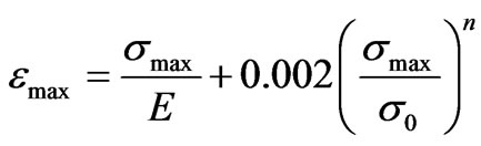
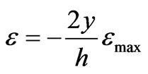 (4)
(4)
emax is the maximum strain produced at the cross section. In most cases, it will not be valid to consider that the neutral plane still passes through the cross-section centroid (an iterative procedure to locate its position will be required), but, if the cross section has a double symmetry along the horizontal and vertical axis, then the neutral plane will not change its position.
Recasting Equation (3) into strain terms
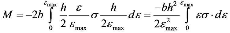 (5)
(5)
But in Equation (1) the strain is given as a function of the stress (and not vice versa), then Equation (5) can be expressed in stress terms as
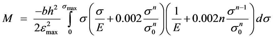 (6)
(6)
After making the integral of Equation (6), the follow ing equation for M is obtained
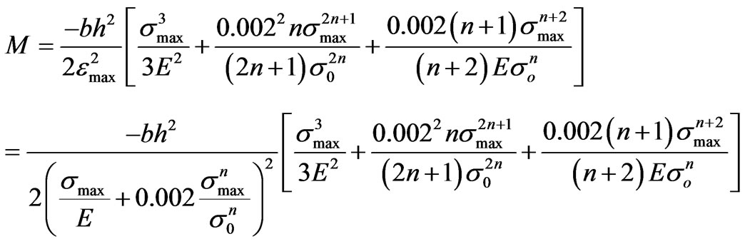 (7)
(7)
Equation (7) allows computing de maximum stress in a section once the applied bending moment at this section is known. The applied bending moment depends on the geometry of the beam, loads… but not of the material that the beam is made of. This Equation (7) is not linear, so an iterative, numerical procedure should be used. If, for example, a Newton-Raphson is to be used, it is convenient to have an explicit expression for its derivative with respect to the maximum stress in the section [9, Press et al.]
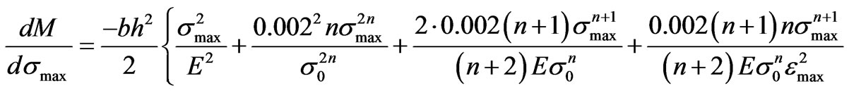
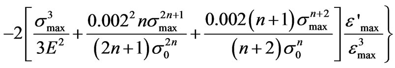 (8)
(8)
where
 (9)
(9)
and
 (10)
(10)
Figure 3 shows a 3-dimensional plot of the evolution of the maximum bending moment (vertical axis) for a square cross section (12.5 × 12.5 mm) in steel (E = 210 GPa, n = 10) with a yield strength (ep = 0.2%) of 600 MPa. Square symbols are plotted at increments of the maximum stress of 10 MPa until fulfilling Considère’s condition (plastic instability, 890 MPa).
1.3. Of a Cantilever Beam
For a horizontal cantilever beam of length L, that support a vertical load at its free end F, the applied bending moment varies along its length as
 (11)
(11)
x represents the position along its length. For example, the maximum moment occurs at its fixed end, x = 0, Mmax = FL. For a particular beam of length L = 1 m and an applied load F = 10 kN, the maximum moment is 10 kN×m. For a rectangular cross section of width b = 40 mm and depth h = 40 mm, it is possible to solve iteratively Equation (7) for the maximum stress at this section. The initial guess might be obtained neglecting the elastic contribution in Equation (7) (introducing E = ¥):
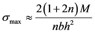 (12)
(12)
In the example case, it results in 656 MPa. Introducing this first guess into Equation (7) a bending moment is obtained (9.367 kN×m, smaller than the imposed one). Now the derivative in Equation (8) (dM/ds = 2.243 ×10⁻⁵ m3) can be used to refine the solution (s max = 685.7 MPa).
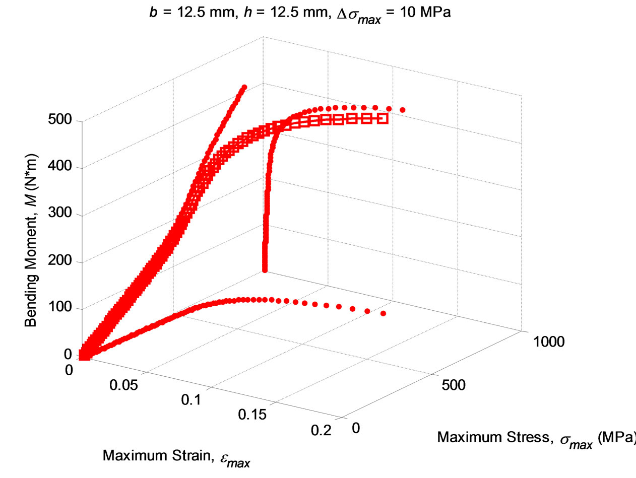
Figure 3. Evolution of the bending moment versus the max. stress and max. strain in steel plate having 12.5 mm × 12.5 mm cross section, E = 210 GPa, s0 = 600 MPa, n = 10. Dots correspond to maximum stress increments of 10 MPa, from 0 to 890 MPa.
Introducing this maximum stress in the material constitutive Equation (1), the maximum strain at this section (at the top or its bottom is obtained) is obtained: emax = 0.01086.
Temporarily we shall introduce the moment that will produce the same maximum strain for an elastic material of identical cross section is
 (13)
(13)
We shall call it elastic-equivalent-bending moment. For the example, Meqe = 24.3 kN×m.
Summarizing, at the fixed end of the beam the actual bending moment is 10 kN×m. This moment produces a maximum strain of 0.01086 at the top (or bottom) of this cross section. Identical maximum strain is produced for an elastic beam (of the same geometry and modulus of elasticity), but with a larger moment: Meqe = 24.3 kN×m.
The bending moment, M, is a function of the position along the cantilever beam, x (see Equation (11)). So, the elastic-equivalent moment, Meqe, can be derived for all along the cantilever beam sections. Figure 4 compares the actual and the elastic-equivalent moments for the proposed cantilever beam.
If the strains all along the top and bottom of both beams: the one built of a Ramberg-Osgood material and the elastic one, are identical, so are displacements, angles, maximum deflection… From this point all the computations can be carried out for the elastic beam under the Meqe distribution. For example, the slope (derivative of the vertical displacements, v, with respect to the longitudinal position, x)
 (14)
(14)
For the example, at the free end it results in an angle of 0.149 rad.
The beam vertical deflections
 (15)
(15)
Any numeric integration procedure can be used to compute Equation (15). In the proposed example, the maximum deflection (at the loaded free end, x = L) is vmax = 108 mm. From Equations (14,15) it is clear that the equivalent elastic moment was a convenient conceptual scaffold, but are not actually required; only the maximum strains are needed.
1.4. Circular Rod
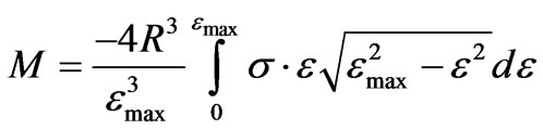
A similar analysis can be carried out for a circular solid cross-section. The bending moment is
 (16)
(16)
Recasting the vertical position into strains, that dis-
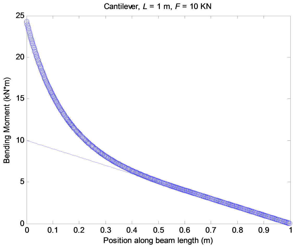
Figure 4. Bending moment for a cantilever beam with a vertical load at its free end (thin line). Distribution along the beam length of the elastic-equivalent bending moment (thick line).
tributes linearly from top to bottom of the section (Euler-Bernoulli’s assumption on plane-sections),
 (17)
(17)
But Ramberg-Osgood equation provides the strain as a function of stress, so, in stress terms (see Equation (18)).
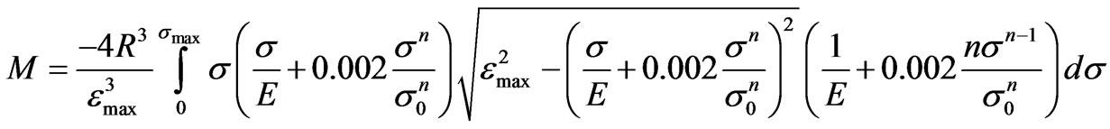 (18)
(18)
That should be solved numerically. Figure 5 shows the evolution of the maximum strain and maximum stress at the solid circular section and the resulting bending moment. For comparison with the previous square section, the diameter is chosen to obtain the same area in the cross section as used in Figure 3 for the square cross section. If both figures are compared (3 and 5, for the square and circular cross sections), the square section supports slightly larger bending moment than the circular one (413 vs. 389 N×m), for a given area and the specified hardening material exponent (n = 10).
1.5. Cantilever Rod
If a rod is used as a cantilever beam, as explained for the rectangular beam, the applied bending moment varies along its length x, see Equation (11). To compute the maximum stress in the different positions along its length, a first numeric estimation can be obtained neglecting the elastic contribution [1].
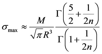 (19)
(19)
For the proposed example, F = 10 kN, L = 1 m, the maximum moment is 10 kN×m, at the fixed cantilever end. If the same cross section, used for the square beam, is distributed in a solid circular geometry, it result in a radius, R = 22.57 mm. Using Equation (19) the first guess for the maximum stress is smax = 694.7 MPa. Using Equation (1) the maximum strain is emax = 0.01197. If these estimations are introduced in the Equation (18) for the moment produced by the longitudinal stresses within the section is 9.469 kN×m, smaller than the applied one (10 kN×m). Any numerical procedure should be used to solve Equation (18). For example, a Newton-Raphson’s; the derivative of the bending moment with respect to the maximum stress is numerically estimated in 2.072 × 10⁻⁵ m3. Per forming iterations it results in a maximum stress smax = 721.5 MPa and the corresponding maximum strain is emax= 0.01607.
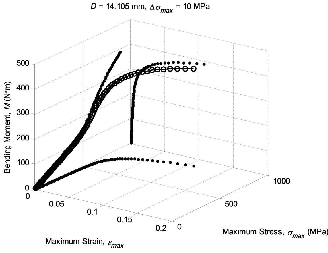
Figure 5. Evolution of the bending moment versus the max. stress and max. strain for a steel rod having a circular 14.105 mm diameter cross section (the same area as for the square section in Figure 3). (E = 210 GPa, s0 = 600 MPa, n = 10). Dots correspond to max stress increments of 10 MPa, from 0 to 890 MPa.
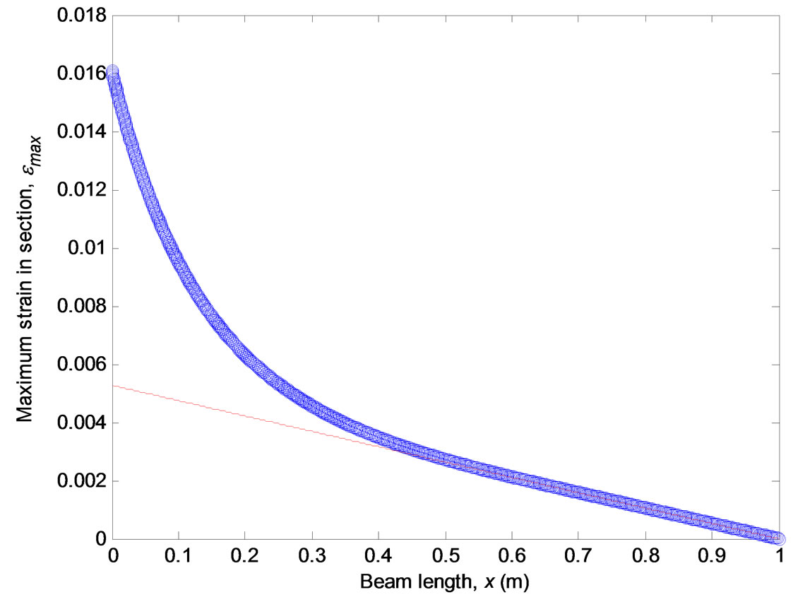
Figure 6. Distribution for the maximum strain along the beam length, from the fixed end to the free and vertically loaded end. Solid circular cross-section. The thin line represents linear elastic case (n = 1).
In the same way, Equation (18) can be solved for the maximum strains along the different cross sections of the beam, as shown in Figure 6.
The beam slopes along its length is computed from
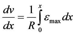 (20)
(20)
And deflections
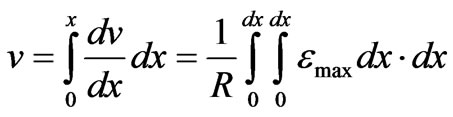 (21)
(21)
Figure 7 represents the beam vertical deflections for the proposed cantilever beam. Note that if the load is positive (upwards), so are the deflections. (Most frequently loads are downwards because of gravity.)
Figure 7 also represents one half of a three point
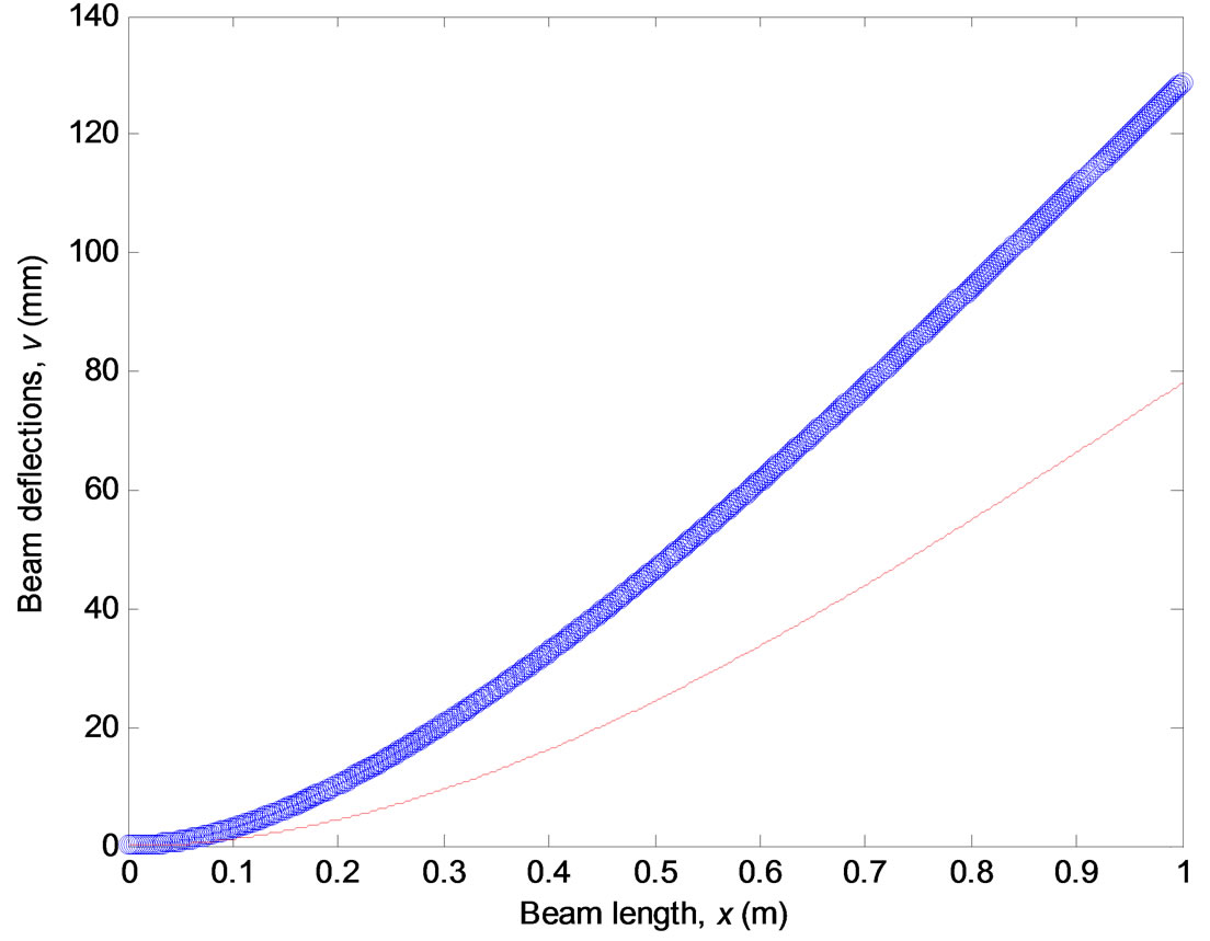
Figure 7. Beam deflections for a cantilever beam, loaded at its free end, with a vertical load of 10 kN (upwards), for a solid circular rod of 45.14 mm diameter (E = 210 GPa, s0 = 600 MPa, n = 10). The thin line represents the linear elastic solution (n = 1).
bending test-piece loaded at its centre with a double load, 20 kN, of identical circular rod (45.14 mm f). These deflections correspond to the displacement observed at the mid-plane and they do not account for probable roll indentations. Note that these indentations are not elastic (but in the case of n = 1) and Hertz’s equations [10,11] are strictly not applicable at the contacts with the rolls.
2. Conclusions
• Non-linear bending of material with a stress-strain behaviour described by Ramberg-Osgood’s equation is described. The maximum bending moments are provided for rectangular and circular solid sections. Equations are derived and a computations procedure is described to obtain beam slopes and deflections.
• Close form, explicit equations are given for the bending moment as a function of the maximum stress in the section, and its derivative with respect to the maximum stress (that is useful for the computer implementation of numerical solutions in a fast and efficient way).
• Two examples are fully described, as close as possible to real tests, under three-point bending; and bending of a cantilever beam with a fixed end, loaded at its free end.
3. Acknowledgments
Thanks are given to Spanish Ministry of Science and Innovation and to the Basque Government for the financial support through the projects MAT2008-03735/MAT and PI09-09, respectively.
REFERENCES
- J. L. Lazagorta and A. Martín-Meizoso, “Non-Linear Bending of Rectangular and Circular Cross-Section Beams,” Under publication.
- J. H. Hollomon, “Tensile Deformation,” Transaction of American Institute of Mining, Metallurgical and Petroleum Engineers, Vol. 162, 1945, p. 268.
- W. Ramberg and W. R. Osgood, “Description of StressStrain Curves by Three Parameters,” Technical Note No. 902, National Advisory Committee for Aeronautics, Washington D.C., 1943.
- H. E. Boyer, “Atlas of Stress-Strain Curves,” American Society for Metals, Ohio, 1988.
- A. Considère, Ann Ponts Chaussee, Vol. 9, 1885, p. 574.
- J. E. Gere and S. P. Timoshenko, “Mechanics of Materials,” 2nd Edition, PWS Publishers, Boston, 1986.
- F. P. Beer, E. R. Johnston Jr. and J. T. DeWolf, “Mechanics of Materials,” 4th Edition, McGraw-Hill, Boston, 2006.
- W. C. Young, “Roark’s Formulas for Stress & Strain,” 6th Edition, McGraw-Hill, Boston, 1989.
- W. H. Press, B. P. Flannery, S. A. Teukolsky and W. T. Vetterling, “Numerical Recipes. The Art of Scientific Computing,” Cambridge University Press, Cambridge, 1986.
- H. Hertz, “Über die Berürung Fester Elastischer Körper,” Journal für die Reine und Angewandte Mathematik, Vol. 92, 1881, p. 156.
- J. E. Shigley and C. R. Mischke, Mechanical Engineering Design, 5th Edition, McGraw-Hill, Boston, 1989.