World Journal of Condensed Matter Physics
Vol.09 No.03(2019), Article ID:93821,15 pages
10.4236/wjcmp.2019.93004
Fermi Energy-Incorporated Generalized BCS Equations for the Temperature-Dependent Critical Current Density and the Related Parameters of a Superconductor for All T ≤ Tc and Their Application to Aluminium Strips
Gulshan Prakash Malik1*, Vijaya Shankar Varma2#
1B-208 Sushant Lok 1, Gurgaon, Haryana, India
2180 Mall Apartments, Mall Road, Delhi, India

Copyright © 2019 by author(s) and Scientific Research Publishing Inc.
This work is licensed under the Creative Commons Attribution International License (CC BY 4.0).
http://creativecommons.org/licenses/by/4.0/


Received: June 25, 2019; Accepted: July 20, 2019; Published: July 23, 2019
ABSTRACT
Presented here are the Generalized BCS Equations incorporating Fermi Energy for the study of the {Δ, Tc, jc(T)} values of both elemental and composite superconductors (SCs) for all T ≤ Tc, where Δ, Tc and jc(T) denote, respectively, one of the gap values, the critical temperature and the T-dependent critical current density. This framework, which extends our earlier study that dealt with the {Δ0, Tc, jc(0)} values of an SC, is also shown to lead to T-dependent values of several other related parameters such as the effective mass of electrons, their number density, critical velocity, Fermi velocity (VF), coherence length and the London penetration depth. The extended framework is applied to the jc(T) data reported by Romijn et al. for superconducting Aluminium strips and is shown not only to provide an alternative to the explanation given by them, but also to some novel features such as the role of the Sommerfeld coefficient γ(T) in the context of jc(T) and the role of VF(T) in the context of a recent finding by Plumb et al. about the superconductivity of Bi-2212.
Keywords:
jc(T) Data for Superconducting Aluminium Strips, Bardeen’s Equation and Kupriyanov-Lukichev Theory for jc(T), Unified Generalized BCS Equations for {Δ, Tc, jc(T)}, T-Dependence of the Sommerfeld Coefficient and Several Other Superconducting Parameters

1. Introduction
Adopting the framework of the Fermi energy (EF)-incorporated generalized BCS equations (GBCSEs), we deal here with the calculation of the critical current density jc(T)—for all T between 0 and Tc—of a superconductor (SC) which is not subjected to any external magnetic field. Specifically, we address here the data obtained by Romijn et al. [1] for superconducting aluminium strips for which it suffices to apply GBCSEs in the scenario where Cooper pairs (CPs) are formed via the one-phonon exchange mechanism (1 PEM). However, with high-Tc SCs in mind, also given here are GBCSEs that enable one to deal in a unified manner with the gaps (Δs), Tc and jc(T) of a composite, multi-gapped SC requiring more than 1 PEM.
The paper is organized as follows. In order to provide a perspective of the conceptual basis of the conventional, multi-band approach (MBA) to the study of the set {Δ, Tc, jc(T)} of a composite SC vis-à-vis that of the GBCSEs-based approach, we include in this section an overview of both approaches. Since the data in [1] are explicable in the conventional approach via both the phenomenological Bardeen equation [2] and the Kupriyanov and Lukichev (KL) [3] theory discussed below, the purpose of this paper is to show that the GBCSEs-based approach provides a valuable alternative explanation of the same data. In the next section are given the EF-incorporated GBCSEs in the scenario when a two-phonon exchange mechanism (2 PEM) is operative. These equations provide a unified framework for the description of the set {Δ2, Tc, j0}, where Δ2 is the larger of the two gaps of the SC. Application of the GBCSEs to the jc(T) data in [1] is taken up in Section 3 where they are also shown to provide the values of several other related T-dependent parameters such as the Sommerfeld coefficient, the effective mass of electrons, their number density, critical velocity, Fermi velocity, coherence length and the London penetration depth. Sections 4 and 5 are devoted, respectively, to a Discussion of our approach and the Conclusions following from it.
1.1. Overview of the Conventional Approach in Dealing with the Set {Δ, Tc, jc(T)} of a Composite SC
The gaps of a hetero-structured SCs are most widely studied via an adaptation of the multi-band approach (MBA) of Suhl et al. [4]. When such a study also deals with a Tc of the SC, which is not always the case, it generally appeals to the Migdal-Eliashberg-McMillan approach (MEMA) [5]. Even though MEMA is cast in the BCS mould of a 1-phonon exchange mechanism (1 PEM) for the formation of CPs, it is employed to deal with such high-Tcs as are observed because it permits the BCS interaction parameter λ to even exceed unity because it is based on an integral equation the expansion parameter of which is not λ, but me/M where me is the electron mass and M the mass of an ion. Insofar as jc is concerned, a plethora of formulae is conventionally employed depending upon the type of the SC (I or II), its size, shape and the manner of preparation—for some such formulae which do not take into account the T-dependence of jc, see [6].
Insofar as jc(T) is concerned, it is empirically known that it has its maximum value at T = 0 and that jc(Tc) = 0. It took considerable time for theoretical attempts to evolve before the observed variation of jc(T) between these limits could be explained. Perhaps the earliest such attempt was due to London, who gave an equation for jc(T) valid at T = Tc, but which failed at lower temperatures because, as was later realized, it did not take into account the effect of the change in the order parameter with current/temperature. The equation for jc(T) given by the phenomenological Ginzberg-Landau (GL) theory marks the next stage in the said evolution. This equation works well close to Tc, but not for much lower temperatures. As is well known, the GL theory reduces to the London theory when the concentration of superconducting electrons is uniformly distributed and that, as was shown by Gor’kov, the microscopic theory in which the energy gap is taken as an order parameter leads to the GL theory near Tc. These brief considerations suggest the need to appeal to the microscopic theory in order to explain the observed variation of jc(T) for all T ≤ Tc. Before we do so, it is relevant to draw attention to a phenomenological equation for jc(T) given by Bardeen [2] post-BCS. This equation, valid for all T between 0 and Tc and obtained by treating the gap as a variational parameter and minimizing the free energy for a given current, is
(1)
Equation (1) is applicable to SCs for which changes in the energy gap with position can be neglected.
Since the thin samples of Romijn et al. [1] satisfied the condition(s) of validity of (1), they applied it to one of their samples and found that it indeed fits their data well. Nonetheless, (1) does not address the core issue of the problem, i.e., to identify the parameters on which jc(T) depends. The knowledge of these is essential because it provides a handle to control jc(T). To unravel what lies beneath the “blanket” of (1), one needs a microscopic theory, viz. the theory given by Eilenberger which is derived from the original Gor’kov theory under the assumption , where ρF is the electrical resistivity of electrons at the Fermi surface and their mean free path. It was shown by KL [3] that for an SC subject to certain constraints, the Eilenberger equations can be further simplified. Since their samples satisfied these conditions, Romijn et al. [1] also employed approximate solutions of the KL equations and found that their data were thus adequately explained.
1.2. Overview of the GBCSEs-Based Approach in Dealing with the Set {Δ, Tc, jc(T)} of a Composite SC
Complementing MBA and presented in a recent monograph [7] is an approach based on the GBCSEs which too has been applied to a significant number of SCs. One of the premises of this approach is that Fermi energy (EF) plays a fundamental role in determining the superconducting properties of an SC. We recall in this connection that the usual BCS equations for the Tc and Δ of an elemental SC are independent of EF because of the assumption that , where k is the Boltzmann constant and θ the Debye temperature of the SC. GBCSEs are obtained via the Matsubara technique and a Bethe-Salpeter equation (BSE) the kernel of which is a super propagator. The latter feature leads to the characterization of a composite SC by CPs with multiple binding energies (|W|s). A salient feature of this approach is that it invariably invokes a λ for each of the ion-species that may cause pairing, whence one has the same λs in the equations for any Δ and the corresponding Tc of the SC—as is the case for elemental SCs. Multiple gaps arise in this approach because different combinations of λs operate on different parts of the Fermi surface due to its undulations. Each of the |W|s so obtained is identified with a Δ of the SC. Thus, as shown in [7] , with the input of the values of any two gaps of an SC and a value of its Tc, this approach goes on to shed light on several other values of these parameters. This is not so for MBA, another feature of which is that even when it is employed to deal with the same SC by different authors, the number of bands invoked is not always the same.
2. EF-Incorporated GBCSEs for the Tc, Δs and jc of a Hetero-Structured SC
2.1. Equations for |W20| (To Be Identified with Δ20, the Larger of the Two Gaps at T = 0), W2(t = T/Tc) and Tc [7]
The equation for |W20| is:
(2)
where
(3)
The equation for |W2(t)| for 0 < t < 1 is:
(4)
where
and the equation for Tc is:
(5)
where
In the above equations, θ1 and θ2 are the Debye temperatures of the ion-species that cause pairing and are obtained from the Debye temperature θ of the SC as detailed in [7] and [8] ; θm is the greater of the temperatures θ1 and θ2, and the variation of chemical potential with temperature has been ignored in order to avoid the situation where we have an under-determined set of equations. Thus, we have assumed that the chemical potential . With the input of |W20|, Tc, and different assumed values of (ρ = 100, 50, 25, 10, 5, etc.), solution of simultaneous Equations (2) and (4) yields, for each value of μ, the corresponding values of the interaction parameters λ1 and λ2.
2.2. Equation for a Dimensionless Construct y0 at T = 0 Which Enables One to Calculate j0 and Several Other Superconducting Parameters
The construct y0 is defined as
(6)
where m*(0) is the effective mass of superconducting electrons at T = 0 and P0 their critical momentum.
The exercise carried out above leads to a multitude of values for the set S = {EF, λ1, λ2}, each of which is consistent with the |W20| and Tc values of the SC. In order to find the unique set of values from among them that also leads to the empirical value of j0 of the SC, we solve the following equation for y0 [9] for each triplet of {EF, λ1, λ2} values:
(7)
where
The operator Re ensures that the integrals yield real values even when expressions under the radical signs are negative (as happens for the heavy fermion SCs).
Corresponding to each value of y0 obtained by solving (6) with the input of {θ, θ1, θ2, EF, λ1, λ2}, we can calculate several superconducting parameters in terms of θ, EF, y0, the gram-atomic volume vg and the electronic heat constant/Sommerfeld coefficient γ0 at T = 0 by employing the following relations, see [8] and for a correction, [10] :
(8)
(9)
(10)
(11)
(12)
where me is the free electron mass and e the electronic charge,
and Ns0 is the number density of CPs and Vc0 their critical velocity at T = 0. Comparison of the j0-values so obtained with the experimental value of j0 then leads to the desired unique set of {EF, λ1, λ2}-values that is consistent with the empirical values of |W20|, Tc, and j0 of the SC.
2.3. Equation for the Dimensionless Construct Which Enables One to Calculate jc(t) and Several Other Superconducting Parameters at t ≠ 0
When t ≠ 0, the equation for y(t) is obtained from [9]
(13)
where
In terms of , we have (12) as:
(14)
where
Each value of y(t) obtained by solving (13) for different values of the set S = {EF, λ1, λ2} leads to the corresponding value of jc(t) via (11), and to the values of the associated parameters via (7)-(10).
3. Explanation of the Empirical jc(t) Values of Aluminium Strips Via GBCSEs
By adding to the RHS of each of the Equations (2), (3), and (4) a term in which λ2 and θ2 are replaced by λ3 and θ3, respectively, the above framework is easily extended to a 3PEM scenario where pairing is caused by three ion-species. On the other hand, in order to deal with the data reported for Aluminium strips in [1] , we need the reduced framework of 1 PEM. This is obtained by putting λ2 = 0 in each of the three equations just noted.
3.1. The j0 Data
Reported in [1] are various superconducting properties for six samples of aluminium strips at T = 0. Among these, Tc and j0 are determined experimentally, whereas values of some other parameters such as coherence length ξ and the London penetration depth λL are model-dependent derived properties.
In order to show how the GBCSEs-based approach works in such a situation, we give below the sequential steps that are followed for Sample 1 in [1].
1) The Tc of the sample is 1.196 K. We take its Debye temperature θ to be 428 K [11]. Employing these values and putting λ2 = 0 (as is appropriate for a 1 PEM), solution of (4) for some typical values of EF are: λ1 = 0.1665 for any value of EF = 10 - 100kθ; λ1 = 0.1666 for EF = 5kθ; λ1 = 0.1670 for EF = 2kθ.
2) For some select pairs of {EF, λ1} values obtained above, we now solve (6) for the corresponding value of y0 and obtain the following results (in the parentheses are given the {EF, λ1} values): y0 = 149.8 {50kθ, 0.1665}; y0 = 149.9 {25kθ, 0.1665}; y0 = 149.9 {10kθ, 0.1665}; y0 = 149.6 {5kθ, 0.1666}; y0 = 149.5 {2kθ, 0.1670}.
3) For each of the above pairs of {EF, y0} values, we now calculate j0 via (11). For this purpose, besides the value of θ, we require the values of γ0 and vg which are taken as: γ0 = 1.36 mJ/mol-K2 [11] , vg = 10 cm3/gram-atom. The results in A/cm2 with the corresponding {EF, y0} values given in parentheses are: 2.37 × 10⁷ {50kθ, 149.8}, 1.49 × 10⁷ {25kθ, 149.8} 8.09 × 10⁶ {10kθ, 149.9}, 5.11 × 10⁶ {5kθ, 149.6}, 2.77 × 10⁶ {2kθ, 149.5}.
4) Among the above values, j0 = 1.49 × 10⁷ A/cm2 corresponding to {EF = 25kθ, y0 = 149.8} is closest to the experimental value of 1.53 × 10⁷ A/cm2. By fine-tuning the value of EF and repeating the above exercise, we find that the experimental value of j0 is obtained exactly when EF = 26kθ = 0.959 eV and y0 = 149.8.
5) With EF fixed at this value, we can find W10 via (2) (with λ2 = 0).
6) With EF and y0 of the sample fixed as above, we can calculate the values of s(0), Ns(0), and Vc0 via (7), (8) and (10), respectively, and the Fermi velocity VF0 at T = 0 via the relation
(15)
Besides these parameters, we can now also calculate the coherence length ξ0 at T = 0 via
(16)
and the London penetration depth λL0 at T = 0 via
(17)
where units for m* and ns are electron-volt and cm−3, respectively, e = (137.03604)−1/2, cm = 5.067728861 × 10⁴(ħc) eV−1 and, for convenience of the reader, we have inserted the requisite factors of ħ and c in order to obtain the value of λL0 in cgs units. The results of these calculations are given in Table 1, which also gives similar results for the remaining five samples dealt with in [1].
3.2. The jc(t) Data
Insofar as jc(t) is concerned, Romijn et al. [1] have given results for one of their samples (Sample 5) in their Figure 4, which is a plot of their experimental values of along with their counterparts as obtained via the phenomenological Bardeen Equation (1) and the KL theory [3]. It follows from this

Table 1. For the samples employed in [1] , the T = 0 values of various superconducting parameters obtained via the procedure detailed in Section 3.1.
graph that the absolute experimental values of jc(t) are given fairly accurately by
(18)
where .
We recall that j0 of Sample 5 in our approach was calculated via the following values of the associated parameters: θ = 428 K, Tc = 1.356 K, λ1 = 0.1701, EF = 12.6kθ, y0 = 132.0, γ0 = 1.36 mJ/mol K−2, and vg = 10 cm3/gram-atom. In order now to calculate jc(t) for this sample, we need to take into account the T-dependence of all these parameters. It seems reasonable to assume that among them, θ, EF and vg retain the values employed for them at T = 0. This assumption enables us to calculate y(t) for any “t” via (13) (with λ2 = 0); the resulting values are given in Table 2. We could now calculate jc(t) if we knew γ(t), but about which we have no information. However, we know that the heat capacity of an SC has a marked non-linear dependence on t as discussed, e.g. in general in [12] and for superconducting Ga in ( [13] , p. 411). We are hence led to calculate γ(t) with the input of jc(t)—rather than the other way around—via the following equation
(19)
the LHS of which for any “t” is taken to be given by (17) and the RHS is calculated via (11) with the input of y(t) obtained by solving (13). These values of γ(T) are included in Table 2. Considered together with the values of y(t), they will be shown below to provide a microscopic justification of Bardeen’s phenomenological Equation (1). It is also remarkable that y(t) and γ(t) enable one to obtain quantitative estimates of several other t-dependent superconducting parameters, viz., s(t) = m*(t)/me, ns(t) = Ns(t)/Ns0, vF(t) = VF(t)/VF0, vc(t) = Vc(t)/V0, ξr(t) = ξ(t)/ξ0, and λLr(t) = λL(t)/λL0. The plots of these are discussed below.
4. Discussion
1) The T-dependence of γ(T) in the context of jc(t) is a new feature of the approach followed here. We recall that, as is well known, γ is usually defined via the equation
Table 2. Obtained as detailed in Section 3.2, values of y(t) and γ(t) corresponding to the experimental values of jc(t) for Sample 5 in [1] for 0 ≤ t ≤ 1.
(20)
where Cp (Cv) is the heat capacity of the SC at constant pressure (volume) at very low temperatures (<10 K). The experimental data are usually plotted in the form Cv/T vs. T2, which yields an intercept equal to γ and a slope equal to 464.6/θ3. The generally reported values of γ in the literature, e.g. in [11] , obtained in this manner correspond to T = 0. It should also be noted that the simple relation (19) is invalid when the magnetic and nuclear contributions may be significant and, importantly, that γ is directly proportional to N(EF), the density of states of electrons at the Fermi level. The latter of these features implies that we are taking into account the T-dependence of N(EF) via γ(T).
2) It was assumed above that among the five parameters that are required for the calculation of jc(t) via (11), we need to take into account the T-dependence of only two of them, viz., y and γ. Since the T-dependence of jc(t) is then governed by , we give for Sample 5 in [1] a plot of R(t) vs. t in Figure 1, where γ(t) and y(t) are obtained via solutions of (18) and (13), respectively. Included in this figure is a plot of the ratio vs. t, which is seen to be almost indistinguishable from the plot of R(t). It therefore follows that our approach based on the microscopic BSE provides a detailed theoretical justification of the phenomenological Bardeen Equation (1) for jc(t).
3) In the approach followed in [1] , while both jc(0) and jc(t≠0) depend on e, Tc, VF, ρF and , the expression for the latter requires additional parameters as is seen from the Appendix in [1]. In the approach followed in this paper, no such additional parameters are required to deal with jc(t≠0); one simply invokes, where applicable, the T-dependence of the parameters on which jc(0) depends, viz. e, θ, y0, γ0, vg and EF. The two approaches may therefore be said to complement each other.

Figure 1. For Sample 5 in [1] : plots of as obtained via solutions of (18) and (13), respectively, and of .
4) The expression for jc(0) in [1] depends on VF, which is not so in the GBCSEs-based approach where jc(0) depends on Vc(0). Nonetheless, it is interesting to note that the value of VF in [1] is assumed to be 1.36 × 108 cm/s for all samples and is not T-dependent whereas, in the approach followed here, it differs from sample to sample and is T-dependent. For Sample 5, it varies between (2.07 - 6.95) × 107 cm/sec for 0 ≤ t ≤ 1. For this sample, the values of ξ0 and λL0 too differ in the two approaches: while reported in [1] for these parameters are, respectively, the values 1.32 × 10⁻⁴ cm and 1.10 × 10⁻⁴ cm, the corresponding values determined by us are 2.39 × 10⁻⁵ cm and 1.00 × 10⁻⁵ cm.
5) Given in Figure 2 are the plots of w1(t), s(t) and ns(t) vs. t for Sample 5 in [1]. Among these, even though the plot of w1(t) is obtained via an EF-incorporated GBCSE with EF = 12.6kθ, it is very similar to the plot one obtains for Δ(T)/Δ0 for an elemental SC via the usual BCS equation sans EF. While we could not find any experimental data for the parameter for the SC under consideration, we draw attention to a plot of this parameter for Pb and Ta given in (Figure 7 of [12] ). This plot covers temperatures up to about 120 K and therefore does not specifically shed light on the behavior of s(t) in the superconducting state. Nonetheless, it is notable that it displays a parabolic decrease for a major part of the range of temperatures over which it is plotted. As for ns(t), as shown in Figure 2, we find that a good analytic fit to the values calculated by us is provided by , which is at variance with the result of the simple two-fluid model where . However, it is also well known that, factually, T-dependences of superconducting parameters often differ from those following from the simple two-fluid model ( [11] , p. 48).
6) In the context of Figure 3 which is the plot of the reduced fermi velocity vF that our approach has led to, we draw attention to a paper by Plumb et al. [14] who have reported that “Associated with this feature (a kink-like feature observed at extremely low energy along the superconducting node in Bi-2212), the Fermi velocity scales substantially—increasing by roughly 30% from 70 to 110 K. The temperature dependence of the feature suggests a possible role in superconductivity, although it is unclear at this time what mechanism(s) may lead to this low-energy renormalization”. We are hence led to suggest that Figure 3 provides both: a plausible explanation that Plumb et al. sought for their result and a validation of our approach.

Figure 2. For Sample 5 in [1] : clockwise, solid lines represent w(t) = W1(T)/W10, s(t) = m*(T)/me, and ns(t) = Ns(T)/Ns0 calculated via, respectively, (3), and the T-generalized (7) and (8). For values of W10, s(0) and Ns0, see Table 1. The dotted plot overlapping s(t) is the analytic fit to it obtained via s1(t) = (1 − t2); the plot overlapping ns(t) is a similar plot obtained via .

Figure 3. Plot of the reduced fermi velocity corresponding to Sample 5 in [1]. The dotted plot overlapping it is obtained via .
7) Both ξr(t) and λLr(t) are known to diverge at t = 1, which is a feature also reflected in our Figure 4 and Figure 5. It is thereby seen that for the former parameter, provides a good fit to ξr(t), whereas a similar fit for the latter parameter is provided by .
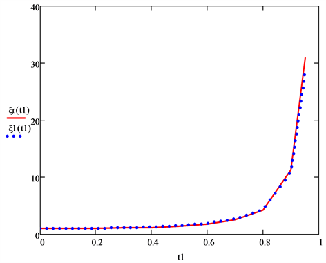
Figure 4. For Sample 5 in [1] , the solid line is the plot of the reduced coherence length as obtained via theory in this paper. The overlapping plot is obtained via .

Figure 5. For Sample 5 in [1] , the solid line is the plot of the reduced London penetration depth as obtained via theory in this paper. The overlapping plot is obtained via .
8) As concerns the rather accurate numerical fits that we have obtained for the values of various empirical parameters associated with jc, it is remarkable that each of them is found to vary as some power of (1 − t2). Viewed in conjunction with (1), it provides another example of the deep physical insight that Bardeen had without the benefit of a detailed microscopic theory governing jc.
5. Conclusions
It has been shown above that the GBCSEs-based approach provides a valuable alternative to the explanation of the Romijn et al.’s jc(T) empirical data for superconducting Al strips based on the KL [3] approach derived from the Eilenberger equations which, in turn, follow from the microscopic Gor’kov theory when certain simplifying assumptions are made. Unique features of the GBCSEs-based approach are: 1) by appealing to the jc(0) value of an SC, it leads to a unique value of EF that enables one to deal with its {Δ, Tc, jc(T)} values in a unified framework, 2) with EF thus fixed, appeal to the jc(t) values of the SC leads to a new finding about how γ(t) varies with t, which is then shown to lead to (3 quantitative estimates of several T- and EF-dependent superconducting parameters, viz., s(t), ns(t), vc(t), vF(t), ξr(t) and λLr(t). It is remarkable that one can obtain these results by remaining within the ambit of the mean-field approximation, i.e. by employing the model (constant) BCS interaction “−V”, which for (6) in the scenario of 1PEM is operative only when , and vanishes otherwise ( [7] , p. 117); for (2), (3) and (4), the corresponding constraints on V are obtained by putting in these inequalities and are identical with those in the usual BCS theory.
As was mentioned above, a plethora of formulae is known in the literature for calculating jc of an SC, depending upon its type (I or II), size, shape and the manner of preparation. The application of EF-incorporated GBCSEs herein, and to a variety of other SCs in [8] (with a correction in [10] ), suggests that the EF of an SC subsumes most of these properties.
We conclude by noting that work is in progress to further generalize the GBCSEs given here to deal with the pragmatic situation where the SC is in a heat bath in an external magnetic field, i.e. when both T and H are non-zero—a procedure for which has been given in [15].
Conflicts of Interest
The authors declare no conflicts of interest regarding the publication of this paper.
Cite this paper
Malik, G.P. and Varma, V.S. (2019) Fermi Energy-Incorporated Generalized BCS Equations for the Temperature-Dependent Critical Current Density and the Related Parameters of a Superconductor for All T ≤ Tc and Their Application to Aluminium Strips. World Journal of Condensed Matter Physics, 9, 47-61. https://doi.org/10.4236/wjcmp.2019.93004
References
- 1. Romijn, J., Klapwijk, T.M., Renne, M.J. and Mooij, J.E. (1982) Critical Pair-Breaking Current in Superconducting Aluminum Strips far below Tc. Physical Review B, 26, 3648-3655. https://doi.org/10.1103/PhysRevB.26.3648
- 2. Bardeen, J. (1962) Critical Fields and Currents in Superconductors. Reviews of Modern Physics, 34, 667-681. https://doi.org/10.1103/RevModPhys.34.667
- 3. Kupriyanov, M.Y. and Lukichev, V.F. (1980) Temperature Dependence of Pair-Breaking Current in Superconductors. Soviet Journal of Low Temperature Physics, 6, 210.
- 4. Suhl, H., Matthias, B.T. and Walker, L.R. (1959) Bardeen-Cooper-Schrieffer Theory in the Case of Overlapping Bands. Physical Review Letters, 3, 552-554. https://doi.org/10.1103/PhysRevLett.3.552
- 5. McMillan, W.L. (1968) Transition Temperature of Strong-Coupled Superconductors. Physical Review, 167, 331-344. https://doi.org/10.1103/PhysRev.167.331
- 6. Malik, G.P. (2013) On a New Equation for Critical Current Density Directly in Terms of the BCS Interaction Parameter, Debye Temperature and the Fermi Energy of the Superconductor. World Journal of Condensed Matter Physics, 3, 103-110. https://doi.org/10.4236/wjcmp.2013.32017
- 7. Malik, G.P. (2016) Superconductivity: A New Approach Based on the Bethe-Salpeter Equation in the Mean-Field Approximation (Series on Directions in Condensed Matter Physics Book 21). World Scientific, Singapore. https://doi.org/10.1142/9868
- 8. Malik, G.P. (2016) On the Role of Fermi Energy in Determining Properties of Superconductors: A Detailed Comparative Study of Two Elemental Superconductors (Sn and Pb), a Non-Cuprate (MgB2) and Three Cuprates (YBCO, Bi-2212 and Tl-2212). Journal of Superconductivity and Novel Magnetism, 29, 2755-2764. https://doi.org/10.1007/s10948-016-3637-5
- 9. Malik, G.P. (2017) A Detailed Study of the Role of Fermi Energy in Determining Properties of Superconducting NbN. Journal of Modern Physics, 8, 99-109. https://doi.org/10.4236/jmp.2017.81009
- 10. Malik, G.P. (2018) Correction to: On the Role of Fermi Energy in Determining Properties of Superconductors: A Detailed Comparative Study of Two Elemental Superconductors (Sn and Pb), a Non-Cuprate (MgB2) and Three Cuprates (YBCO, Bi-2212 and Tl-2212). Journal of Superconductivity and Novel Magnetism, 31, 941-941. https://doi.org/10.1007/s10948-017-4520-8
- 11. Poole, C.P. (2000) Handbook of Superconductivity. Academic Press, San Diego.
- 12. Kresin, V.Z. and Zaitsev, G.O. (1978) Temperature Dependence of the Electron Specific Heat and Effective Mass. Soviet Physics JETP, 47, 983.
- 13. Kittel, C. (1974) Introduction to Solid State Physics. Wiley Eastern, New Delhi.
- 14. Plumb, N.C., et al. (2009) Low-Energy (< 10 meV) Feature in the Nodal Electron Self-Energy and Strong Temperature Dependence of the Fermi Velocity in Bi2Sr2CaCu2O8+δ. https://arxiv.org/pdf/0903.4900.pdf
- 15. Malik, G.P. (2010) On Landau Quantization of Cooper Pairs in a Heat Bath. Physica B, 405, 3475-3481. https://doi.org/10.1016/j.physb.2010.05.026
NOTES
*Formerly of the School of Environmental Sciences, Jawaharlal Nehru University, New Delhi, India. #Formerly of the Department of Physics and Astrophysics, University of Delhi, Delhi, India.