International Journal of Astronomy and Astrophysics
Vol.4 No.1(2014), Article ID:43407,10 pages DOI:10.4236/ijaa.2014.41001
Non-Trivial Linkup of Both Compact-Neutron-Object and Outer-Empty-Space Metrics
Luboš Neslušan
Astronomical Institute, Slovak Academy of Sciences, Tatranská Lomnica, Slovakia
Email: ne@ta3.sk
Copyright © 2014 by author and Scientific Research Publishing Inc.
This work is licensed under the Creative Commons Attribution International License (CC BY).
http://creativecommons.org/licenses/by/4.0/


Received 30 October 2013; revised 30 November 2013; accepted 9 December 2013
ABSTRACT
In 2011, Chinese researcher Ni found the solution of the Oppenheimer-Volkoff problem for a stable configuration of stellar object with no internal source of energy. The Ni’s solution is the nonrotating hollow sphere having not only an outer, but an inner physical radius as well. The upper mass of the object is not constrained. In our paper, we contribute to the description of the solution. Specifically, we give the explicit description of metrics inside the object and attempt to link it with that in the corresponding outer Schwarzschild solution of Einstein field equations. This task appears to be non-trivial. We discuss the problem and suggest a way how to achieve the continuous linkup of both object-interior and outer-Schwarzschild metrics. Our suggestion implies an important fundamental consequence: there is no universal relativistic speed limit, but every compact object shapes the adjacent spacetime and this action results in the specific speed limit for the spacetime dominated by the object. Regardless our suggestion will definitively be proved or the successful linkup will also be achieved in else, still unknown way, the success in the linkup represents a constraint for the physical acceptability of the models of compact objects.
Keywords:Ultra-Compact Objects; Hollow Spheres; Classical General Relativity; Oppenheimer-Volkoff Problem

1. Introduction
It is known that the final stage of a star that spent all storage of its nuclear fuel is either a white dwarf or a neutron star. Or, if the mass of dying star exceeds the Oppenheimer-Volkoff limit, the object is believed to eternally collapse to its center, i.e. it becomes a black hole. The mass limit between the stable and unstable neutron objects was found, at the first time, by Oppenheimer and Volkoff in 1939 who solved the appropriate equations [1] . Hereinafter, we refer to this problem, with the original set of equations considered, as to the OppenheimerVolkoff (OV) problem. In more detail Oppenheimer and Volkoff considered a cool, non-rotating object consisting of neutrons. Its gravity was described by the Einstein field equations adopted for the spherical symmetry of the problem [2] -[4] . The quantities characterizing the object’s interior were calculated from the equation of state for the cold, degenerated, Fermi-Dirac neutron gas published by Landau as well as by Chandrasekhar [5] [6] . Oppenheimer and Volkoff used the form of equations given by Chandrasekhar (a more detailed description is provided in Section 2).
A few years ago, in 2011, Chinese scientist Ni published the solution of the equations figuring in the OV problem for a stable object without any upper mass limit [7] . The original feature of this solution is the existence of an inner physical surface of corresponding object. We therefore will call this object as “hollow sphere”. Soon after the Ni’s paper was published, Mei independently considered the hollow-sphere concept (he was the first who used the term “hollow sphere”) as well as the solid spheres and described the metrics for the object of a constant density [8] . He however did not deal with the metrics of adjacent empty space.
The description of any stable compact object can be regarded as complete if not only the behavior of state quantities, but the behavior of the metrics in its interior as well as in the surrounding empty space is given. The linkup of the interior and empty-space metrics appears to be a non-trivial task. It this paper, we deal with this problem.
The paper is divided into six sections. In Section 2, we recall the basic equations of the OV problem. In Section 3, we discuss the suitable initial values entering the numerical integration of the equations. We demonstrate that the asymptotic solution of these equations for the radial distance  implies an infinite magnitudes of pressure and energy density. Thus, a realistic solution for a stable object must start in a distance larger than zero. It means that the object has to have an inner surface and is, therefore, the hollow sphere. Because of this reason, we deal only with the metrics linkup in the case of hollow sphere in Sections 4 and 5. The concept of the hollow sphere seems to harbor all stable neutron objects, also those of neutron-star size.
In Section 4, we attempt to link up the interior and empty-space metrics for the set of obvious conditions and assumptions and demonstrate that it is not possible in this case. In Section 5, we suggest a solution of this problem and outline the consequences of one new, modified assumption. Some concluding remarks are presented in Section 6.
2. Outline of the Problem of Stable Configuration
Before any further study, let us summarize the basic set of the equations in the OV problem. We recall, the equations describe a spherically symmetric, non-rotating object, which consists of a cold, degenerated, mono-particle (neutron), Fermi-Dirac gas.
The gravitational field inside the object is described by the Einstein field equations [2] [3] . These can be simplified, to find a static solution for the case of spherical symmetry, to form
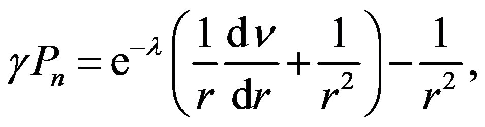 (1.1)
(1.1)
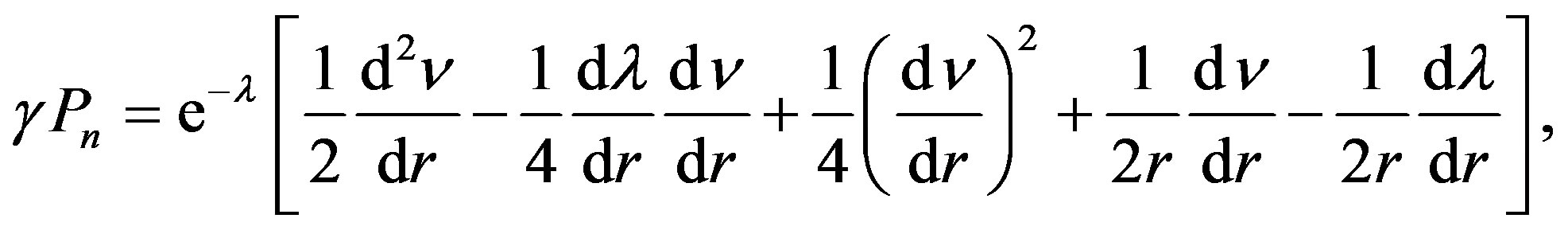 (1.2)
(1.2)
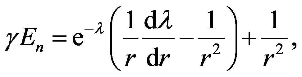 (1.3)
(1.3)
with the line element defined by
 (1.4)
(1.4)
in the spherical coordinate system r,  , and
, and , where
  is the pressure and En is the energy density of the degenerated neutron gas,
  and
and  are the functions depending on the radial coordinate
  in the static case, and c is the relativistic speed limit (equal to the velocity of light) [4] . We denoted
 , where
  is the gravitational constant. In purpose, we use the SI units throughout the paper. The field equations yield the condition of hydrodynamical equilibrium
 (1.5)
(1.5)
The condition gives the pressure gradient balancing the gravity. If there is a larger gradient in the gas, the object expands and vice versa. Oppenheimer and Volkoff re-wrote this condition to form
 (1.6)
(1.6)
where the function  was established as
 (1.7)
(1.7)
With the help of field equations, the derivative of this function with respect to  can be given as
 (1.8)
(1.8)
To find if the requirement on the pressure gradient set by relation (1.6) can be satisfied, one can again follow Oppenheimer and Volkoff who utilized the equation of state for the degenerated Fermi-Dirac gas in the form presented by Chandrasekhar [6] (Appendix). Specifically, they considered the formulas for energy density  and pressure
  converted to forms
 (1.9)
(1.9)
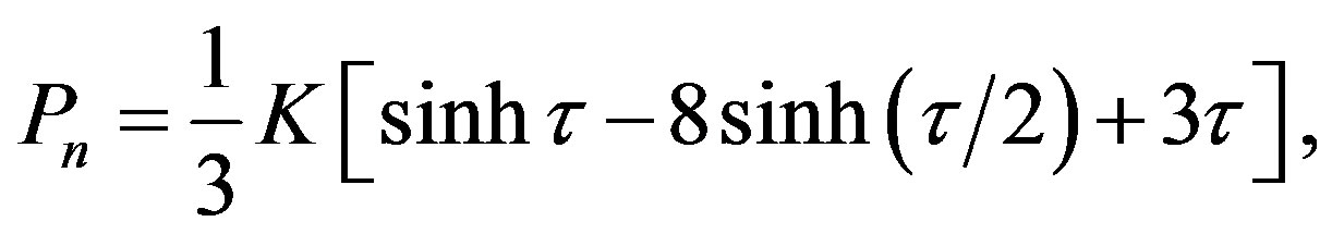 (1.10)
where 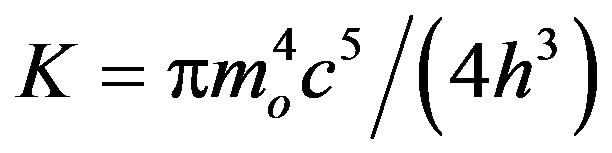 and
and
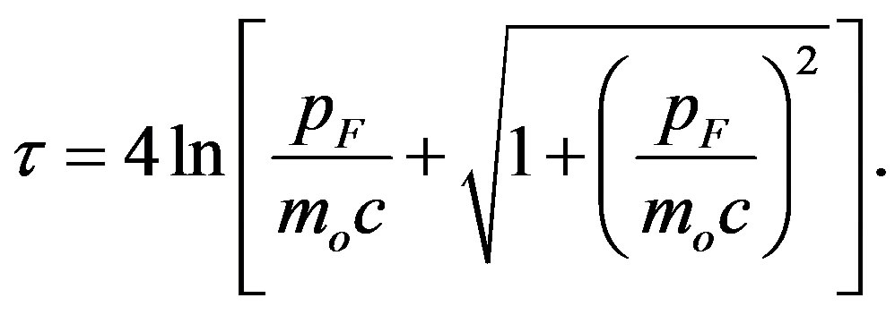 (1.11)
Denotation used:  is the rest mass of the gas constituents (neutrons), h is the Planck’s constant, and
  is the Fermi impulse. The inverse relation to (1.11) is
 .
.
According to Oppenheimer and Volkoff, the pressure gradient,  , is proportional to
 (1.12)
They also re-wrote Equation (1.8) with the help of formula (1.9) to
 (1.13)
Equations (1.12) and (1.13) give the derivatives of  and u in the Schwarzschild coordinates. However, the effective gradient of pressure (Equation (1.6)) is the differential of the pressure,
  , divided by the proper element of the radial coordinate. If one wants to replace the Schwarzschild element
  with the proper element
 , the exchange
  (see, e.g., [9] , p. 605) or
  has to be made. Equation (1.6)
then changes to
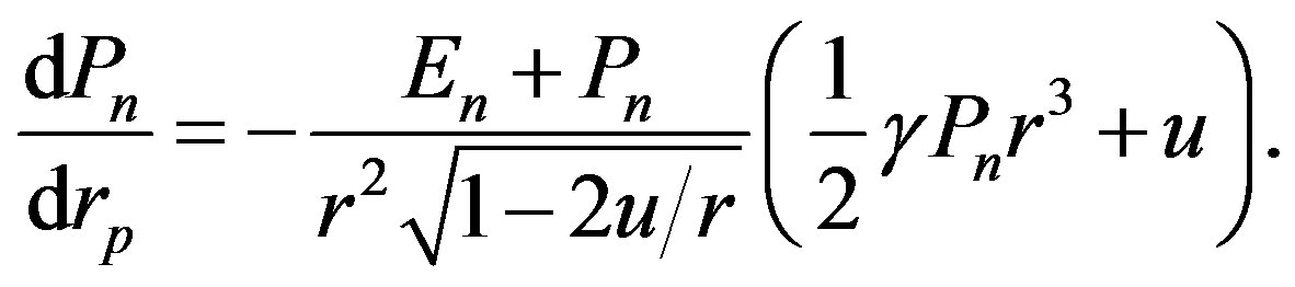 (1.14)
In the calculation of , the correction factor
  occurs in both left-hand and right-hand sides of the appropriate equation, therefore it eliminates itself and Equation (1.12) remains unchanged.
The behavior of  -component of metric tensor can be gained integrating equation
 (1.15)
simultaneously with Equations (1.12) and (1.13). Equation (1.15) is derived from Equation (1.1), in which  is replaced with the form containing the function
  with respect to relation (1.7). The choice of initial value
  entering the numerical integration is arbitrary, when a solution independent on, e.g., outer Schwarzschild (OSCH, hereinafter) metrics is calculated. If one seeks a convergence of
  to the OSCH solution in
 , a relevant value of
  has to be searched for in an iteration.
The internal (heat) energy of, e.g., the Sun is negligible in comparison to its rest energy. According to the model of stellar structure published in [10] (Table 7 in [10] ), the heat energy inside the solar body can be estimated . The rest energy of the Sun equals
  and is, therefore, many orders of magnitude larger than the heat energy. A similar ratio between the internal and rest energies can be assumed for other normal stars and other non-compact objects. It however appears that the internal energy of the objects described by the solutions found here can be so large that it exceeds, several times, the objects’ rest energy. Consequently, the mass of the object, M, largely exceeds its rest mass,
 . Therefore, we need to distinguish between both masses.
The object’s rest mass can be calculated as
 (1.16)
and its total mass is given by
 (1.17)
where  is the rest mass of neutron and
  is the number density given by relation
 (1.18)
3. Starting the Numerical Integration
Differential Equations (1.12) and (1.13) can be integrated numerically. To find the physically acceptable behavior of the quantities occurring in these equations, one must, however, choose the suitable set of initial values entering the integration.
Assuming that the energy density is a function of pressure (e.g. , where
  is a constant and
  is a real number), Oppenheimer and Volkoff started the numerical integration at the origin of coordinate system, i.e. at
 , where they assumed the finite initial values
  and
and  of integrated quantities [1] . Ni however showed that the origin can be a conflict point for the starting [7] . In the following, we present another argumentation against the start in this point.
For , we can assume an asymptotic form of solution of
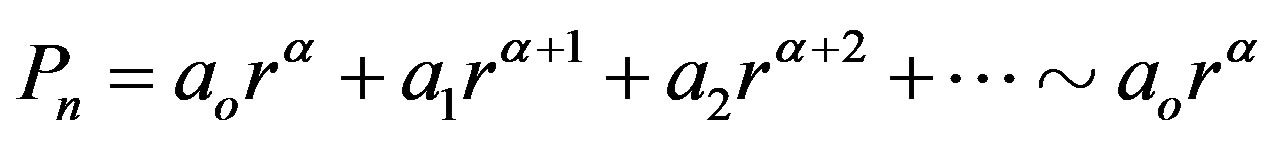 ,
,
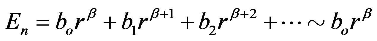 , and
, and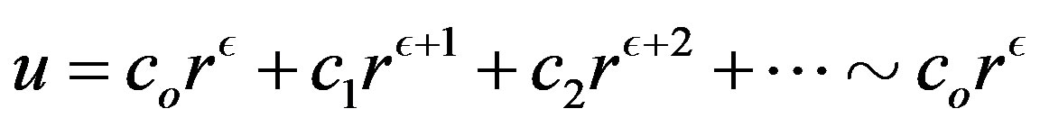 , where coefficients
 ,
,  , and
, and 
 as well as indices
 ,
,  , and
, and  can acquire arbitrary real values. Supplying the assumed power series for
 ,
,  , and
, and  to Equations (1.14), (1.8) and neglecting the higher than the first terms, we obtain the equations
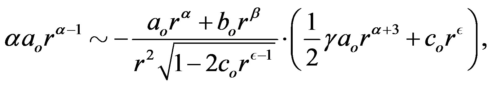 (1.19)
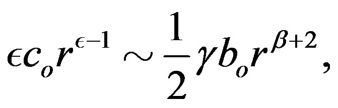 (1.20)
from which a constraint on the indices ,
,  and
and  can be derived. We divide Equation (1.19) by
  and Equation (1.20) by
 . The new equations, after a simple algebraic handling, are
 (1.21)
 (1.22)
To keep the argument of the square root figuring in Equation (1.21) finite, there has to be valid the condition (i)  (if
(if , then
 ). The terms in the parentheses of Equation (1.21) do not diverge if conditions (i), as well as (ii)
 , (iii)
 , and (iv)
  are valid. Since the left-hand sides of Equations (1.21) and (1.22) are non-zero, one of forms in the conditions (i)
 (iv) has to be equal zero and also condition (v)
  must be valid. Condition (iv) can be re-written as
 , whereby
 . Using (i), we obtain
 . Now, taking into account this last inequality and the re-written form of condition (iv), we have
 . The inequalities in the borders can be satisfied only for (vi)
 .
.
If condition (vi) is valid, then (ii) and (iii) as well as (i) and (iv) become identical. Since one of (i) (iv) must change to the equality equal to zero, either
  or
or . In the first case, i.e.
 , condition (v) implies
  and, according to (vi), also
 . In the second case,
  and, again according to (vi), also
 . It means that
  and
and  when
when . In other words, point
  is singular and, hence, it is inappropriate for starting the numerical integration.
Ni started some integrations in the outer radius,  , of the object. We however regard also this starting point as problematic. In both radii,
  and
and , the pressure (and energy density) is zero. With respect to Equation (1.10) (and Equation (1.9)), quantity
  must also be zero. For
  or
or  andgenerally,
  , forms
  and
and  when
when  in Equation (1.12). But the other form in this relation, fraction
  for
for . So,
. So,  for
for , therefore the numerical integration has to start in other distance than r = Rin or r = Rout. Numerically, we can closely approach to
  (integrating inward) and
  (integrating outward), but it is impossible to reach these borders in the correct calculation. (Fortunately, all quantities we are interested in converge to a finite value when we approach these points, therefore the above mentioned circumstance has no practical impact on our analysis.)
In conclusion, the numerical integration of Equations (1.12) and (1.13) should start in a distance , which is
  assuming an initial value of Fermi impulse
  and initial value
 , which is constrained by the necessity of positive argument of square root in relation (1.14). This necessity implies
 . To perform the integration, we use the Runge-Kutta method.
Hyperbolic sines and hyperbolic cosines set a high demand on the precision of the calculations when the numerical integration is performed. We found that the common Fortran “double” precision (REAL*8) is insufficient to make the integration for some combinations of the input parameters. (One can do a simple test changing the length of integration step. Using the Fortran double precision, the resultant behaviors of corresponding integrated quantities were not the same for various step lengths.) C-computer-language “long double” precision appears to be a minimum demand to perform the integration with a satisfactory precision.
4. Search for Continuity
In this section, we start to deal with the continuity of metrics in the outer radius of object. Since we consider the spherically symmetric object, only the diagonal components of metric tensor are non-zero. The spherical symmetry also causes that the corresponding transverse components of the tensor,  and
and , for the interior of hollow sphere and surrounding empty space are identical. Hence, we need to link up only the radial and time components,
  and
and , in
, in .
.
Within our study, we calculated (doing also a lot of iterations) several hundreds of the solutions, for a large variety of input parameters. The obtained solutions indicate a possibility of existence of small, white-dwarfstarsized stable compact neutron objects with their mass distributed as a hollow sphere. (Some of them have internal density sufficient for keeping the neutrons stable!) One can also find some solutions at the currently estimated critical limit between the neutron stars and black holes. Or, the masses considerably exceed the upper limiting mass of neutron stars, but—we emphasize—all these solutions are for the stable objects. The range of masses of stable neutron objects is quite large.
There are the solutions for the stable objects with the outer radii above the classical event horizon, but also for the objects below this horizon. (Below, we distinguish between the common, well-known, i.e. “classical” event horizon and “modified” event horizon.)
The examples of the behavior of  and
and  components of metric tensor in two solutions are shown in Figures 1(a) and 1(b), respectively. The corresponding behavior of density, calculated as
 , is shown in Figure 1(c). The mass of the object described by the first (second) solution is
 and the rest mass equals
 . While the first example is related to the object with its outer physical radius smaller than the corresponding classical Schwarzschild gravitational, Rg, the outer radius is larger than Rg in the second example. Thick curves in Figures 1(a) and 1(b) show the behaviors in the interior of each object. The dotted curve shows the behavior of
  as well as
  in the corresponding OSCH solution for the second object.
When the solution for the hollow sphere is calculated using an ad hoc set of constants ,
,  ,
,  , and
, and  entering the numerical integration in its beginning, like in the cases shown in Figure 1, the function
  related to the interior of object has never any common point with
  of the corresponding OSCH solution. The analogous functions
  have either no common point or the OSCH-solution function crosses that for the object’s interior in an arbitrary point of the latter. Making an iteration, we can find such a value of input constant
  that the crossing of both
  functions occurs just in the distance
 , i.e. we can achieve a linkup of both functions we searched for. However, it appears that this linkup is not continuous.
In Figure 1(b), the increasing part of each function  corresponds to the gravity acting inward and the decreasing part to the gravity acting outward from the origin of the used Schwarzschild coordinate frame (center of the object). In the interval corresponding to the inward acting gravity,
  decreases with decreasing r, i.e. this behavior is similar to the corresponding Schwarzschild
 . However, the decrease does not continue to the value
  for
for . Instead, there is a turn-point, where the gravity (net gravity, more exactly) is zero and its action becomes oriented outward, in shorter distances. In each of these shorter distances, e.g. in
 , the summary mass accumulation in the external half-space with respect to an observer situated in
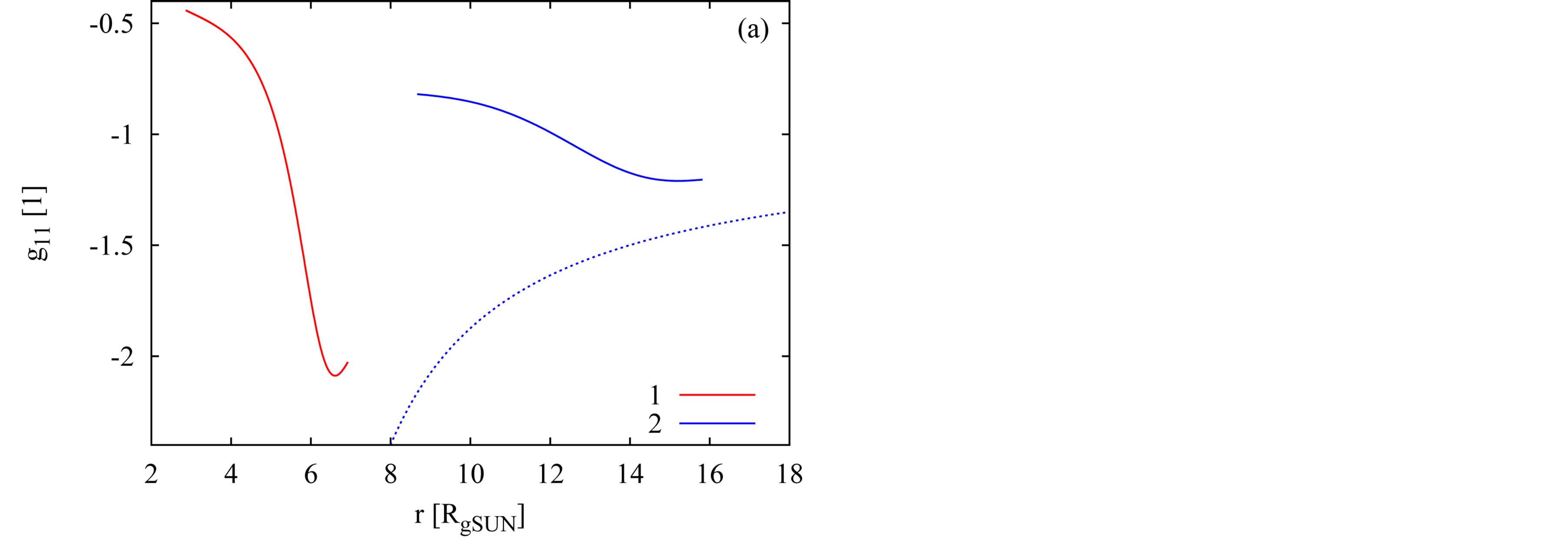
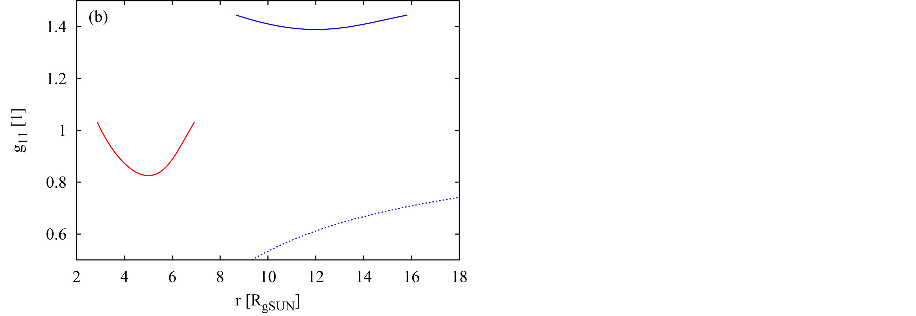
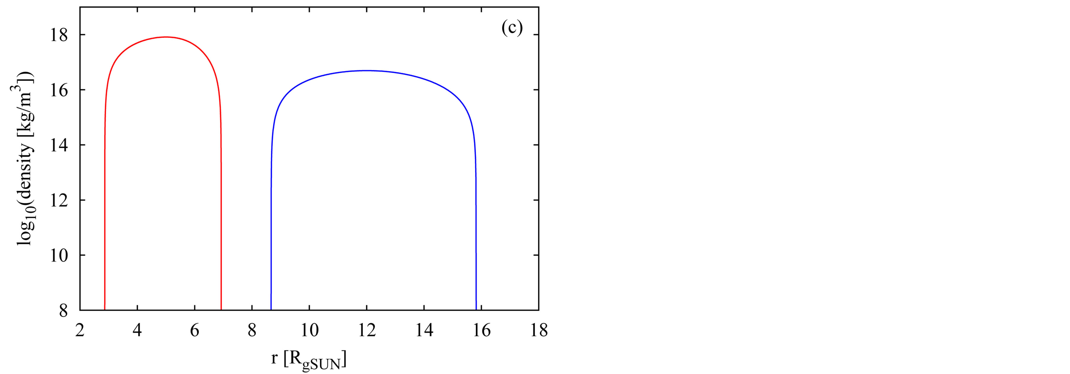
Figure 1. Two examples of the behavior of components g11 (plot a) and g44 (b) of metric tensor and the internal density (c) inside the compact objects described by the concept of hollow sphere. The dotted curves in plots (a) and (b) show the behavior of g11 and g44 in the OSCH solution for the second object.
distance  is obviously measured larger than that measured in the supplementary internal half-space.
The above mentioned change in the orientation of the gravitational action implies the following, important, general-relativistic effect. Let us consider a thin, perfectly spherically symmetric material layer. We know that the net gravitational force on a test particle inside the layer is zero in the Newtonian approximation. In a strongly curved, relativistic field, the net gravity on the particle is not zero, but the particle is attracted to the nearest point of the layer.
The consequence of this non-zero net gravity is a qualitatively new feature of the relativistic object in comparison with an object described by the Newtonian physics: the existence of the inner surface. The surface is the essential feature of the hollow-sphere concept. To well accept this concept for the physical description of real objects, it is worthy to discuss the mechanism of the occurrence of the inner physical surface. Let us again consider the thin, homogeneous, spherically symmetric layer, but now consisting of a gas. The pressure gradient forces the gas to expand outward as well as inward. The outward oriented expansion can be stopped when the pressure gradient is balanced by the gravity in both Newtonian physics and general relativity. This is the mechanism of the occurrence of the outer physical surface of gaseous objects as common stars, gaseous planets, or neutron stars. The inward oriented expansion cannot however be stopped in the Newtonian physics, since the net gravity inside the layer is zero and there is, therefore, no force to balance the pressure gradient in this case. The gas has to fill in the whole interior of the layer.
However, as was evidenced above, the gravitational attraction inside the layer is larger than zero and oriented toward the nearest point of the layer in the strongly relativistic spacetime. So, there is the agent that can balance the pressure gradient and can, therefore, yield the inner surface. Our inspection of several tens of found solutions indicates that the gravity not only can, but it always balances the gradient of pressure and creates the inner surface. The mechanism of occurrence of inner physical surface in general relativity is essentially the same as the mechanism of the occurrence of outer physical surface.
The linkup of function  can be achieved by the finding of the appropriate value of input constant
  entering Equation (1.15). Can we also achieve a linkup of function
  by the finding of an appropriate combination of input constants
 ,
,  (implying
 ), and
  entering the system of Equations (1.12) and (1.13)? Let us now deal with this question.
From the mathematical point of view, the link up occurs when the function  describing the metrics in the object will equal its counterpart in the OSCH solution in
 . According to Equation (1.7), the former can be given as
 , where we denoted
 . The OSCH solution gives
 . Now, it is easy to demonstrate that these functions equal each other if 2uout = Rg.
A search, if the equality  can occur, in the whole, three-dimensional phase space of initial values
 ,
,  , and
, and  would be difficult. We reduce the number of the initial parameters to two starting the integration in the maximum of
  -behavior, i.e. in the point where
 . According to Equation (1.12), the first possibility to obey this demand is the equality
  or
or . One can prove that this is the condition for the (double) local minimum of function
  (assuming the physical demand that
 ). The local minima occur in borders
  and
and . The second possibility to obey demand
 , which we utilize, is
 (1.23)
Now we calculate the solutions for the sequences of initial  and
and .
.
To find if  can acquire the value of
 , we construct the dependence of ratio
  on the input value of Fermi impulse,
  , for several input distances,
  , and inspect if the value of this ratio equals unity. Since the integration of Equations (1.12) and (1.13) always starts in the distance of the maximum pressure, i.e. with the value of input
  given by Equation (1.23), also
  is included into the considered set of initial values and, thus, the whole phase space of reasonable combinations of
 ,
,  , and
, and  is considered in fact.
The resultant dependencies of  on
on  for a set of
  are shown in Figure 2 (each curve is for the given value of
 , which is indicated, in the solar gravitational radii
 , in the top left corner of the figure. The ratio is always a monotonous, increasing function of
  and approaches unity only in the limit of
 , which implies the limit
 . So, the ratio seems to never equal to unity in the case of the object of a finite mass. In other words, there is no combination of initial parameters, which would lead to such a
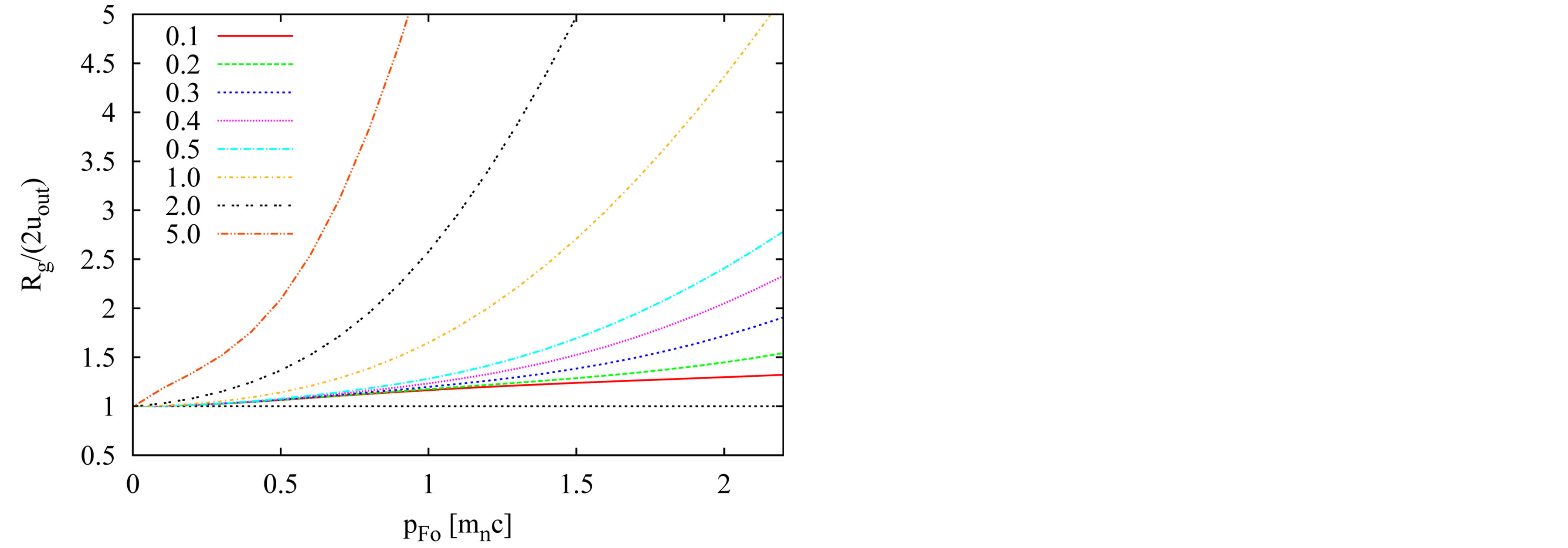
Figure 2. The dependence of ratio Rg/(2uout) on the value of input constant pFO entering the numerical integration in the beginning for several sequences of solutions of Equations (1.12) and (1.13). The given sequence (curve in graph) is characterized by the same value of another input parameter ro. Its value is written in the left upper corner of plot. The unit of ro is the solar gravitational radius, . The dotted horizontal line shows the limit, unity, that is attempted to be reached.
behavior of  that its end-point in
  would be, at the same time time, the point of the function
  of the OSCH solution. A suggestion to remove this problem and to achieve the continuity of
  in
in  is presented in the next section.
5. New Gauging in the Outer Schwarzschild Solution
In this section, we present a suggestion of how to achieve the perfect linkup of the metric tensor describing the spacetime in the interior of hollow sphere with that in the corresponding OSCH solution in distance . Namely, the discontinuity in the
  and
and  linkup found in the previous section, if not removed, would be a serious problem not only in course of an acceptability of newly found solutions for stable objects, but also in the course to physically accept the OSCH solution itself, because the active agent curving the spacetime is the mass accumulation in the object. So, the object and the solution describing its structure are primary and the description of surrounding spacetime should be an extension of the solution for the object.
It however seems that the discontinuity can be only a problem occurring due to our not completely appropriate requirements in the gauging of the integration constants in the OSCH solution. In the OV problem, there is the system of three differential equations of the first degree (Equations (1.1)-(1.3)), which imply three integration constants. Two of these constants,  and
and , occur in the general form of g11 and g44 components of metric tensor. Specifically,
  and
and . In the process of deriving the solution (see, e.g., [4] ), we obtain equation
 , which gives
 , after its integration. So, it produces the third integration constant,
 . In the gauging of solution, the metrics is demanded to become flat in the limit of
  (free space), i.e.
  and
and .
.
Analyzing in detail the relation for the line element, especially its form (1.4) written in the SI units, we see that the metrics is given not only by the metric tensor, but by the speed limit, c, as well. In the gauging of constant , the implicit assumption that the speed limit is always equal to c is thus comprehended, in addition. The metric tensor obviously describes the curvature and the maximum velocity characterizes the “intrinsic” properties of spacetime. (Or, we can include the factor of
  to
to  -component of metric tensor, which will then converge
  in the limit
 . To retain all components of metric tensor dimensionless, we however prefer the representation with the intrinsic properties.) In the following, let us hypothetically assume that not only the metric tensor, but the intrinsic properties of spacetime and, therefore, the value of the speed limit can be shaped by a material object. Quantitatively, a significant change of the intrinsic properties can be expected at the relativistic, compact objects.
Splitting the characteristics of spacetime to its curvature and intrinsic properties, the requirement of the flat, Euclidean space for  can also be satisfied for
 . If we convert this constant to another constant,
  , via relation
 , the line element (1.4) for the non-zero
  (or
(or ) can be given as:
 (1.24)
Product  in the last term of this relation can be regarded as the limiting velocity in the spacetime shaped by the object to which constant
  (and therefore
 ) is related. We denote this new limiting velocity by
 .
.
Changing the limiting velocity, the Schwarzschild gravitational radius has to also be changed, from  to
to , whereby
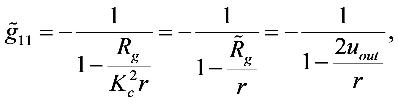
 . In the outer radius of object, the modified function
  is, thus, equal to
 . Since this must be, at the same time (according to the requirement of continuity), equal to
 , the quadrate of
  is equal to
 (1.25)
Ratio  can be calculated from the quantities M and uout obtained from the numerical integration. In all solutions obtained, it was valid that
  (see Figure 2. Hence, Kc > 1 and, consequently,
  and
and . We note, the components
  and
and  of the OSCH solution for Kc > 1 can be given as
 (1.26)
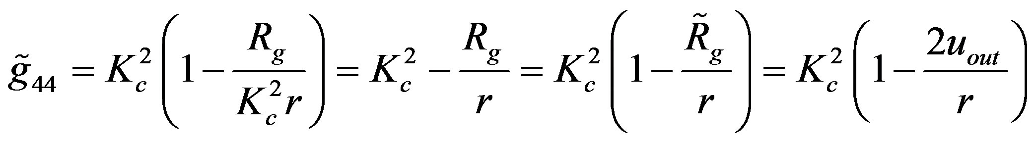 (1.27)
Interestingly, if the correction of the limiting velocity about factor  is done, it is not only possible to find the point of the OSCH-solution function
  identical to the point of this function for the hollow sphere in
 , but the linkup of both functions is the continuous function. The derivatives of
  with respect to r of both OSCH-solution and hollow-sphere functions equal each other. In addition, the continuity also appears in the case of the linkup of component
 . The success of the linkup of
  and
and  is illustrated in Figure 3. It is intriguing that the modification of the single assumption (
 is changed to
 ) enables to achieve three partial result: (i) it removes the displacement in
 , (ii)
  becomes the continuous function in
  as well as (iii)
  becomes the continuous function in
 .
.
Furthermore, it appears that the continuity exists not only in the case of objects with , but for those with
  as well. The example is the first solution shown in Figure 3. The occurrence of the continuity for
  is possible due to the fact, noticed empirically, that there is always valid the inequality
 . According to the found solutions, the object never shrinks below the “modified” event horizon.
The radial component of acceleration due to gravitational force in the limit of weak, Newtonian field, is given as  when the unit of speed
  and as
  when the SI units are used. It appears that this acceleration is the same regardless the speed limit is
  or
or . Namely,
 and
and 
i.e. we obtain the same result in both cases.
6. Concluding Remarks
Every model of compact object should also provide a description of the metrics of spacetime in its interior as well as in the neighboring empty space. Otherwise the model cannot be regarded as complete and, therefore, physically well-acceptable. Considering a simple model of non-rotating, stable, compact neutron object, we pointed out the serious problem concerning the linkup of metrics at the outer physical surface.
Nevertheless, a definitive conclusion based only on our result would be premature. The concerning scientific community does not widely know the problem, at the moment. As far as we know, the linkup has not been tried to be achieved in a variety of existing models of neutron stars, either. Nor was it considered at the spinning compact objects. In principle, there are two following ways in course to definitively solve the problem of the linkup. Our work contributes to both ways.
(1) The universal relativistic speed limit will be retained. It supposes that some still unknown way of the successful linkup will be found in the future. It will be possible if the discontinuity of the metrics in  is not
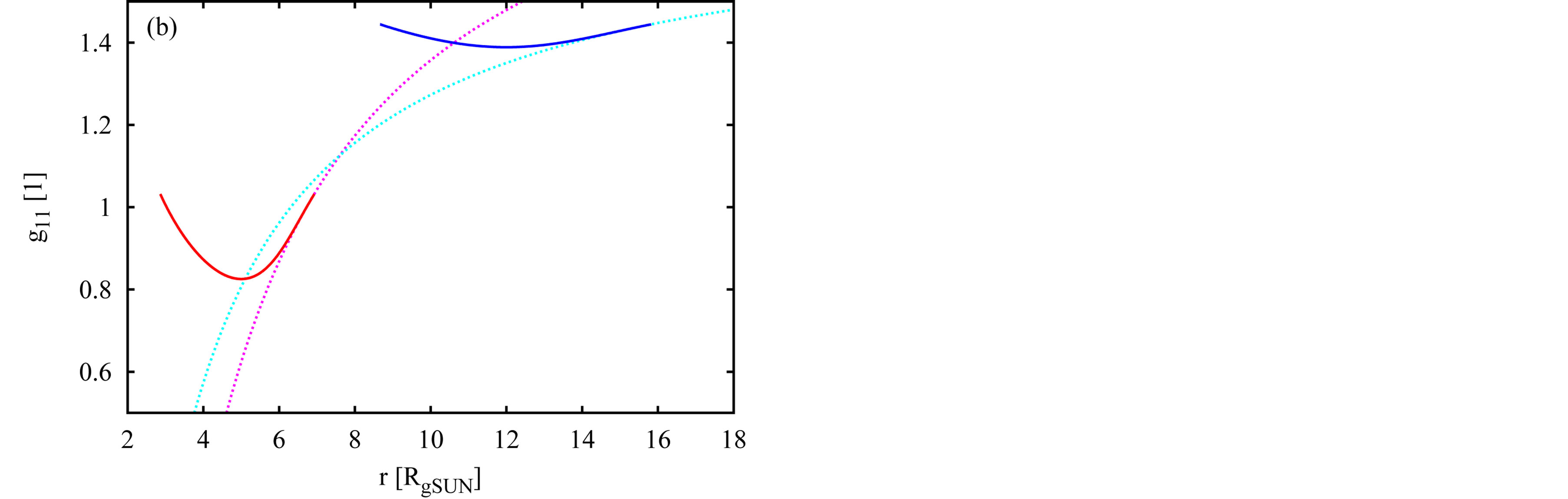
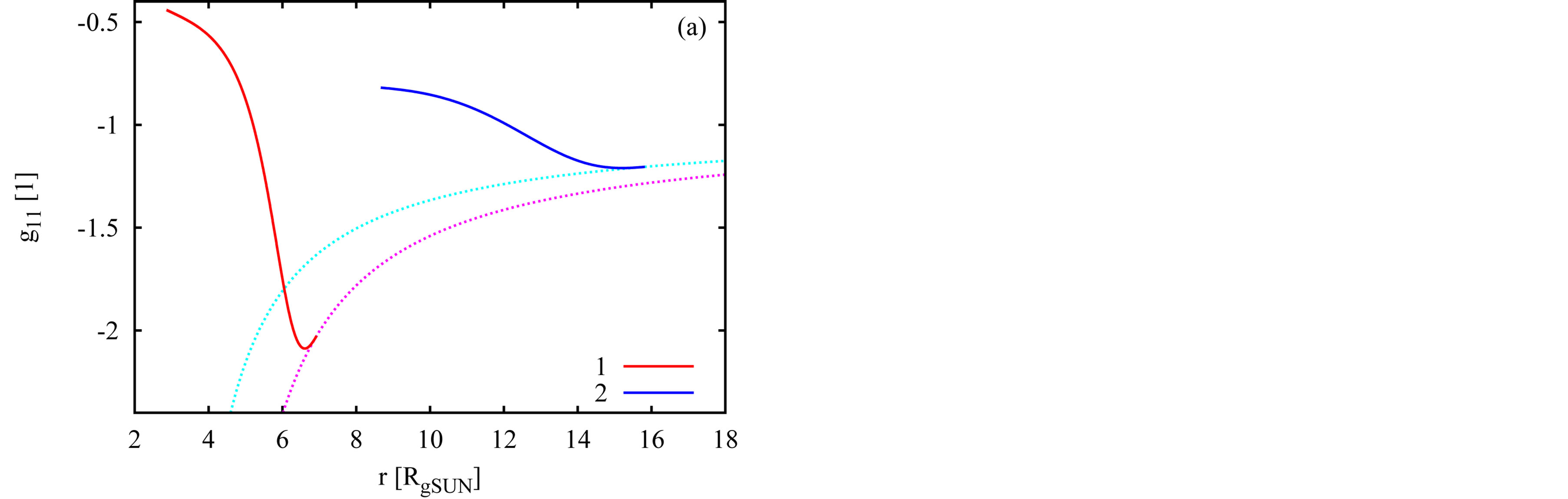
Figure 3. Two examples of the successful linkup of components g11 (plot a) and g44 (b) of metric tensor inside two compact objects described by the concept of hollow sphere (thick curves) with g11 and g44 in the OSCH solution (thin, dotted curves), in r = Rout.
attribute of every possible model of the compact object. The demand on the success in the linkup is then an important constraint for the models of compact objects. It discriminates between the realistic and pure theoretical (toy) models. The specific speed limit for given compact object suggested in Section 5 is, likely, only a theoretical possibility.
(2) The continuous linkup can be achieved only in the way we suggested in Section 5. Since we showed how to make the continuous linkup, it is no longer any problem in this case. However, we have to accept the serious fundamental consequence: there is no universal relativistic speed limit, but every compact (and not only compact, in principle) object shapes the adjacent spacetime and this action results in the specific speed limit for the spacetime dominated by the object. As well, we also have to accept the further consequences of this consequence. These will however be a subject of future research if this, second, alternative is more proved to be the reality.
Acknowledgements
This work was supported by VEGA—the Slovak Grant Agency for Science, grant No. 0011 and by the Slovak Research and Development Agency, project No. APVV-0158-11.
References
- Oppenheimer, J. and Volkoff, G. (1939) On Massive Neutron Cores. Physical Review, 55, 374-381. http://dx.doi.org/10.1103/PhysRev.55.374
- Einstein, A. (1915) Die Feldgleichungun der Gravitation. Sitzungsberichte der Preussischen Akademie der Wissenschaften zu Berlin, 844-847.
- Einstein, A. (1916) Die Grundlage der Allgemeinen Relativitätstheorie. Annalen der Physik, 354, 769-822. http://dx.doi.org/10.1002/andp.19163540702
- Tolman, R.C. (1969) Relativity, Thermodynamics, and Cosmology. Clarendon Press, Oxford.
- Landau, L. (1932) On the Theory of Stars. Physikalische Zeitschrift Sowjetunion, 1, 285-288.
- Chandrasekhar, S. (1935) The Highly Collapsed Configurations of a Stellar Mass (Second Paper). Monthly Notices of the Royal Astronomical Society, 95, 207-225.
- Ni, J. (2011) Solutions without a Maximum Mass Limit of the General Relativistic Field Equations for Neutron Stars. Science China, Physics, Mechanics, and Astronomy, 54, 1304-1308. http://dx.doi.org/10.1007/s11433-011-4350-9
- Mei, X. (2011) The Precise Inner Solutions of Gravity Field Equations of Hollow and Solid Spheres and the Theorem of Singularity. International Journal of Astronomy and Astrophysics, 1, 109-116. http://dx.doi.org/10.4236/ijaa.2011.13016
- Misner, C.W., Thorne, K.S. and Wheeler, J.A. (1997) Gravitation. W. H. Freeman and Company, New York.
- Turck-Chieze, S., Cahen, S., Casse, M. and Doom, C. (1988) Revisiting the Standard Solar Model. Astrophysical Journal, 335, 415-424. http://dx.doi.org/10.1086/166936