Journal of Transportation Technologies
Vol.07 No.03(2017), Article ID:76699,19 pages
10.4236/jtts.2017.73016
Suitability of the Euler’s Spiral for Roadside Clearance in Order to Provide Stopping Sight Distances
Timur Mauga
Department of Civil and Environmental Engineering, UAE University, Al-Ain, UAE

Copyright © 2017 by author and Scientific Research Publishing Inc.
This work is licensed under the Creative Commons Attribution International License (CC BY 4.0).
http://creativecommons.org/licenses/by/4.0/


Received: March 9, 2017; Accepted: May 29, 2017; Published: June 1, 2017
ABSTRACT
The AASHTO’s guideline for geometric design, also known as the green book, requires that the inside of horizontal curves be cleared of obstructions to sight lines in order to provide sufficient sight distances. Recently, innovative use of Euler’s spiral for determination of clearance offsets has been proposed. However, suitability of the offsets as minimum criteria has not been evaluated. This paper presents comparison between the proposed offsets and minimum offsets determined with the computational method suggested in the green book. Results of comparison show that offsets determined with innovative use of the Euler’s spiral are always longer than minimum values determined with the computational method. The differences in lengths of the two sets of offsets increase with decrease in curve radii. Therefore, on sites with large radii offsets determined through innovative use of the Euler’s spiral may be implemented in the field since the offsets are only slightly longer than minimum offsets. On sites with short radii some offsets on tangent sections are very long such that they result in extra cleared areas that will not accommodate sightlines. The areas that do not accommodate sightlines may result in unnecessary extra earthwork costs where highways are located in cut zones. Additionally, it has been suggested in this paper that designers also consider other curves, including elliptical arcs, for roadside clearance envelopes. One advantage of elliptical arcs is that they are flexible to align with boundaries of clear zones on tangent sections regardless of sizes of radii of horizontal curves. Besides, most offsets to elliptical arcs are comparable to those determined with the green book’s computation method. An example of design chart has been presented for practitioners to use. The chart is for minimum offsets needed to provide a given sight distance while gradually transitioning clearance from boundaries of clear zones on tangent sections.
Keywords:
Roadside Clearance, Clearance Offsets, Sightline Offsets, Clearance Envelope, Sight Distance

1. Background
Part of design of safe highways is provision of sufficient sight distance. On long tangent sections sufficient sight distances are naturally provided since sightlines are completely accommodated within travel lanes. But at horizontal curves sightlines have to be chords to the curves for drivers to have sufficient sight distance. Where there are high roadside objects on the inside of the curves the objects block sightlines and negatively affect sight distances. For that reason, the AAHTO’s guideline for geometric design [1] , famously known as the green book, and other design codes require that objects on the inside of horizontal curves be cleared so as not to block sightlines. The green book’s analytical model for the minimum extent of clearance is presented by Equation (1). This equation is on page 3-109 presented as Equation 3 - 36 in the current green book.
 (1)
(1)
where
M is the minimum roadside clearance offset measured from driver path;
R is the radius of driver path;
S is the stopping sight distance (SSD);
The offset obtained with Equation (1) is suitable for middle sections of curves that are longer than stopping sight distance. The middle sections start at PC + 0.5S and end at PT − 0.5S, where PC is the point of curvature or the beginning of curve and PT is the point of tangency or the end of curve. The reason Equation (1) is suitable for the section between PC + 0.5S and PT − 0.5S is that the equation is for maximum ordinates from sightlines to curved segments whose lengths are equal to stopping sight distance. Naturally, maximum ordinates are middle ordinates that bisect both the segments and the sightlines. However, the green book suggests that the offset be used all over horizontal curves on the ground that the offset is only slightly and mostly insignificantly larger than actual offsets needed for sections near beginnings and ends of curves. Few studies [2] [3] [4] [5] have found that minimum offsets required near beginnings and ends of curves are significantly smaller than values calculated with Equation (1).
In providing sufficient sight distance the green book is still accurate in its suggestion that M be used all over the curve since that M will guarantee that available sight distances are equal to or greater than stopping sight distances. Also, the suggestion fits well sites whose offsets to boundaries of clear zones on tangent sections are equal to M. Moreover, the suggestion to use M uniformly fits well where horizontal curves are not passing through deep cut zones otherwise use of offsets long as M near beginnings and ends of curves may increase earthwork costs. But the green book is flexible since it suggests that if designers feel that values obtained with Equation (1) are inapplicable they may use the computational method [2] or the graphical method to determine suitable clearance offsets. The procedure for the graphical method for determining minimum offsets has been presented in past studies [3] [4] [5] . In the procedure, an offset at a given location is a horizontal distance from driver path (and normal to the driver path) to the farthest sightline at that location.
The graphical method produces accurate minimum offsets at each location. Accuracy of the method is based on the fact that sightlines on horizontal alignments are oriented the same way actual sightlines are oriented in the field. It is accuracy that got the method recommended by the green book and accepted by practitioners and researchers. Some commercial software packages for geometric design conduct sight distance analyses using the graphical method. Packages that use the method are not mentioned here in order to avoid commercialization.
The assumption based on which the graphical method is conducted is that a subject driver constantly monitors a road segment ahead with length equal to stopping sight distance. The assumption is easy to understand if it is explained in terms of a subject vehicle following another vehicle that is located a distance equal to stopping sight distance and that both vehicles are moving from upstream a curve to its downstream [6] [7] . Locations of the leading vehicle represent minimum safe locations of dangerous objects. The result of the assumption is minimum offsets that guarantee that provided sight distances are equal to or greater than stopping sight distances. The minimum offsets are thus the criteria of acceptance or rejection of provided (or available) offsets.
Despite high accuracy of the graphical method, past studies have reported that the method is tedious and time consuming. Tedium and wastage of time were motivations in those studies to develop design charts for clearance offsets. The charts were developed to analytically reproduce offsets that are equal to offsets determined with the graphical method. An example is the chart developed by Raymond [2] which is also recommended by the current green book. Another example of design charts is the chart developed by Glennon [3] . Although currently there are software packages that can determine clearance offsets on a click of a mouse, the charts are still useful where an engineer cannot access a computer, like on sites, or the computer does not have a routine for the graphical method. The charts are also useful for pedagogical purposes. The only drawback of the two charts is that they are not applicable for sites with curves that are shorter than stopping sight distance.
Recently, Mauga [4] [5] derived equations for offsets that reproduce offsets determined with the graphical method for long and short highway curves. Mauga validated the analytical offsets with offsets determined with the graphical method because the method has been recommended by the green book and accepted by practitioners and researchers. Along with validating the analytical offsets, Mauga compared the analytical offsets with offsets derived from charts that were earlier developed by Raymond [2] and Glennon [3] and found them to match. Mauga also developed a design chart for practitioners to use. Although the chart was developed based on vehicles traveling at constant speed, it was later shown that the chart is also applicable for sites with variable operating speeds [7] . Therefore, the chart by Mauga [4] [5] and earlier charts by Raymond [2] and Glennon [3] are all one and the same and are in perfect agreement with their parent that they mimic (i.e. the graphical method).
The graphical method and its analytical counterparts use curve geometry (i.e. radius and length) and stopping sight distance as input to directly output minimum offsets. These minimum offsets are used as criteria for whether or not to clear a roadside object of given offset. If an offset to a roadside object, which may be referred to as an available offset, is less than the minimum offset then the object has to be removed or the curve has to be redesigned. If the available offset is greater than the minimum offset then the object is left alone since it does not impact sight distance negatively. An example where available offsets are greater than minimum offsets is on approach tangent sections just downstream of PC-S. On the tangent sections significant lengths of sightlines near drivers are accommodated within lanes, making minimum offsets shorter than the available offset to the boundary (i.e. outside edge) of the clear zone. The shorter minimum offsets are usually discarded and the boundary of the clear zone automatically becomes part of the provided clearance envelope.
2. The Problem
There has been recent studies that have proposed use of roadside clearance boundaries or envelopes that are different from clearance envelopes resulting from the graphical method and its analytical charts [2,3]. For example, Ameri et al. [8] assumed that the roadside clearance envelope was a transformed Euler’s spiral that starts at the beginning of a horizontal curve. However, Ameri et al. did not check whether or not that envelope provided at least stopping sight distance at all locations. They could have used the graphical method to conduct that check. Mauga [5] evaluated use of the Euler’s spiral as clearance envelope in the way the graphical method is conducted and found that the Euler’s spiral would provide sight distances that are less than stopping sight distance.
You and Easa [9] proposed innovative use of the Euler’s spiral as a roadside clearance envelope near beginnings and ends of horizontal curves such that the spiral provides sight distances that are at least equal to stopping sight distances. You and Easa [9] also developed design charts for offsets to the Euler’s spiral (also referred to as the innovative envelope in this paper). However, the offsets to the innovative envelope were not compared with accurate minimum offsets determined with models already accepted in practice: minimum offsets derived from Raymond’s chart [2] or minimum offsets determined with the graphical method.
3. Objectives
The main objective of this paper is to analyze suitability of innovative use of the Euler’s spiral as minimum roadside clearance envelope. The analysis indirectly compares offsets to the innovative envelope with minimum offsets to the Raymond’s envelope by comparing available sight distances determined with the innovative envelope and available sight distances determined with the Raymond’s envelope. For both envelopes, available sight distances are determined assuming that there is no vehicle downstream a subject driver such that available sight distances are functions of roadway and roadside geometry only and not functions of space headways. The criterion of suitability of the innovative envelope as minimum clearance envelope is closeness of the envelope’s available sight distances to available sight distances provided by the Raymond’s envelope. The Raymond’s envelope is chosen as basis of comparison since minimum offsets to it are accurate and that the envelope has been recommended by the green book and implemented for longer than 40 years. The comparison is limited to sites with curves that are longer than stopping sight distance. The comparison also considers sites with constant speeds as well as sites with variable speeds. Another objective is to suggest use of elliptical arcs as alternative clearance envelopes.
4. Raymond’s Clearance Envelope
Part of the design chart developed by Raymond [2] for minimum offsets is a line for simple curves whose lengths are equal to or longer than stopping sight distance. The chart provides offsets expressed as fractions of offset M given by Equation (1). The offset fractions or ratios are for a segment from PC-S on the driver path where the offset ratio is zero to PC + 0.5S where the offset ratio is 1. A practitioner using the Raymond’s chart determines offsets by reading offset ratios from the chart then multiplying the ratios with offset M given by Equation (1). There are some offsets that are smaller than the offset to the boundary of clear zone on tangent sections. The smaller offsets are usually discarded and the ones that are equal to or greater than the offset to the boundary of clear zone are implemented in the field. The resulting clearance envelop is a combination of straight boundaries of clear zones on tangent sections and the curved clearance boundary resulting from the implemented offsets. The envelope is also the same as envelopes that result from implementing other models such as Glennon’s chart [3] and Mauga’s chart [4] [5] since all are accurate analytical models of the graphical method. Figure 1 presents the Raymond’s clearance envelope together with the innovative envelope proposed by You and Easa [9] .
5. Sites with Constant Speed
In practice, chosen design speed is used for determining geometric properties of highways. One of the elements that are determined with design speed is stopping sight distance. Since design speed is a fixed value, the resulting stopping sight distance is also fixed for a given grade and coefficient of friction. The value of stopping sight distance is then used to determine roadside clearance offsets so as to accommodate sightlines on the inside of horizontal curves. If the offsets are determined with Raymond’s chart then the resulting available sight distances

Figure 1. Raymond’s and the innovative clearance envelopes.
will be at least equal to stopping sight distance.
To determine available sight distances consider a 70 mph (SSD = 730 ft) highway. At a curve, the inside lane has a sharp radius of 1480 ft and length of 1480 ft. This highway is closer to the metric 110 km/h highway with radius of 414 m presented as an example by You and Easa [9] . In addition to radius and length, the offset to the boundary of clear zone on tangent sections is taken as 12 ft (measured from driver path) for the Raymond’s envelope. The 12 ft offset is small but allowed since the AASHTO’s guide for roadside design [10] states that shy-line offsets presented in the guideline are not critical if they are continuous. For the innovative envelope, the offset to the boundary of the clear zone on tangent sections is calculated as 30 ft, which is the same as the offset at PC − 0.5S following the procedure presented by You and Easa [9] . The 30 ft offset is assumed as the offset to the boundary of the clear zone upstream of PC − 0.5S and downstream of PT + 0.5S since You and Easa [9] did not suggest a transition scheme to small clear zone offsets such as shy-line offsets. The 30 ft offset is equivalent to 21 ft measured from the edge of traveled way. The 21 ft offset is much longer than all shy-line offsets suggested in the AASHTO’s guide for roadside design [10] and offsets that long may be costly to implement in cut zones.
To determine available sight distances for both envelopes, sightlines are made to touch envelopes tangentially (where practical) for each driver location. Figure 2 presents available sight distance profiles for the two envelopes. The figure also presents a profile for the SSD of 730 ft (which is constant due to constant grade and surface friction). Unlike geometry based profiles of available sight distances for the two envelopes, the SSD profile may be considered as a traffic based profile of available sight distance since it is a function of space headway i.e. the subject vehicle is behind a lead vehicle by SSD, and that both vehicles are in motion from far upstream of the curve to far downstream of the curve. This SSD profile is the concept based on which the graphical method and its analytical charts [2] [3] [4] [5] were derived.
In Figure 2, for the innovative envelope, when a driver is within the curve from PC to PT-S the available sight distance is equal to the stopping sight dis tance of
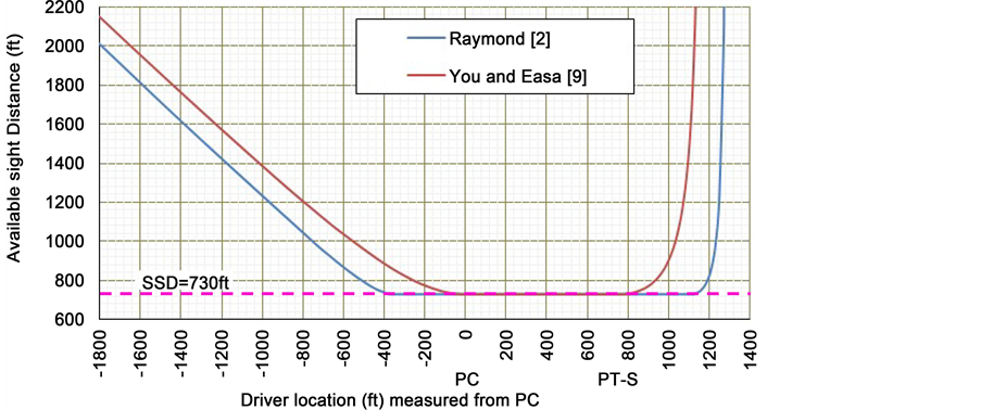
Figure 2. Available sight distance profiles for the innovative and Raymond’s envelopes.
730 ft and the clearance offset is equal to M in Equation (1). Upstream of PC and downstream of PT-S the available sight distances provided by the innovative envelope are greater than those provided by Raymond’s envelope. However, the additional available sight distance on the approach tangent is relatively small given the extra offset of at least 18 ft (i.e. 30 - 12 ft) on the approach tangent.
The 30 ft offset at PC − 0.5S for the innovative envelope is not meant to provide extra clear zone for recovery of out-of-control vehicles. The 30 ft offset at PC − 0.5S is primarily meant to provide space for accommodating sightlines onthe roadside. But sightlines that would touch the innovative envelope tangentially at PC − 0.5S correspond to drivers that would imaginarily be infinitely far upstream while tangent sections have finite lengths. Since tangent sections have finite lengths, no sightline will touch the envelope tangentially at PC − 0.5S and a little downstream of PC − 0.5S. Therefore, the 30 ft offset will not serve its purpose. For example, the sightline that touches the innovative envelope 34.2 ft downstream of PC − 0.5S corresponds to an imaginary available sight distance of 10 miles. Practically, the 10 miles sight distance is unavailable. The reason is that the Earth is curved hence a subject driver cannot see the subject highway curve since the horizon blocks sightlines from the subject highway curve to the subject driver. But it is the imaginary 10 miles and other imaginary longer sight distances that necessitate clearance of 30 ft offsets upstream of PC − 0.5S while the sight distances are practically not fully usable by drivers. The long offsets will thus cause unjustifiable extra earthwork costs upstream of PC − 0.5S where highways pass through cut zones.
To partially reduce the extra earthwork costs near PC − 0.5S and upstream or near PT + 0.5S and downstream, a designer may propose transition of clearance from the straight boundary of the clear zone on tangent sections to the point which splits the innovative envelope into two portions: ineffective portion and effective portion. The ineffective portion is the one either whose available sight distances are impractical (i.e. overlong sight distances like the example of 10 miles presented above) or no sightline touches the portion of the envelope due to tangent sections being short. The effective portion is the one whose available sight distances are practical. On long tangent sections, determination of practical available sight distances should consider the maximum distance at which a driver can recognize a 2 ft high object, bearing in mind that objects appear to apparently diminish in size as distance from an observer increases. Also, on long tangent sections, determination of practical available sight distances should consider sight distances that command response of drivers to the 2 ft high stimulus.
On short tangent sections, determination of practical available sight distances is based only on sightlines touching the envelope tangentially. For example, for the 70 mph highway with 12 ft offset to clear zone boundary on tangent sections, if the approach tangent is equal to stopping sight distance S then 45.36% of the length of the approach spiral just downstream of PC − 0.5S is ineffective (i.e. no sightline touches the envelope tangentially within the 45.36% of the length of the spiral). Only the remaining 54.64% of the length of the spiral provides practical available sight distances. If the approach tangent is 0.5S then only 37.24% of the approach spiral provides practical available sight distances. The effective length of the spiral decreases as the length of the approach tangent decreases, questioning applicability of the innovative envelope on roadsides of winding roads. Figure 3 presents an example of transition from the boundary of clear zone to the innovative envelope on sites with short tangents between reverse circular arcs. The transition line can be straight or an arc that aligns well with the boundary of the clear zone upstream of PC − 0.5S and downstream of PT + 0.5S.
An alternative to transitioning shown in Figure 3 is implementation of the innovative envelope on sites where the offset at PC − 0.5S equals to the offset to the clear zone boundary on tangent sections such that the envelope aligns well with the boundary upstream of PC and downstream of PT. A designer may strategically provide large radii (keeping the intersection angle fixed) such that 67% of the value of M in Equation (1) equals the offset to the boundary of clear zone. For the offset of 12 ft to the boundary of clear zone, a radius of 3700 ft will be sufficient to align the innovative envelope with the boundary. The 3700 ft iswhat You and Easa [9] would consider as maximum radius for use of the inno-

Figure 3. Transition from clear zone to the innovative envelope.
vative envelope for a 70 mph highway with 12 ft offset to clear zone boundary. For sites with radii greater than 3700 ft but less than 5550 ft there still will be the need of clearance downstream of PC − 0.5S and upstream of PT + 0.5S. But You and Easa [9] did not provide solution for that range of radius. It is unclear whether or not it was implied that practitioners use already existing models such as charts developed by Raymond [2] , Glennon [3] , and Mauga [4] [5] or use the graphical method or that radii longer than 3700 ft are not to be used at all since part of the innovative envelope will fall within the clear zone (i.e. innovative offsets will be shorter than offsets to clear zone boundaries).
Suggesting 3700 ft as maximum radius for use of the innovative envelope (for 70 mph and 12 ft clear zone offset) guarantees that always the innovative envelope will lie outside the clear zone on tangent sections. Such restriction implies that there will always be extra earthwork on tangent sections where highways pass through cut zones. Such extra earthwork will add unnecessary extra cost since sight distances provided by the shy-line offset at PC − 0.5S are already greater than stopping sight distances. To avoid such extra cost the 3700 ft should be considered as minimum value. The innovative envelope will thus cross the clear zone boundary. Part of the innovative envelope near PC − 0.5S and PT + 0.5S will be in the clear zone and part of it outside the normal clear zone. Having part of the envelope in the clear zone is not undesirable situation. The length of the envelope laying in the clear zone is actually a proof that nearly the same length of clear zone boundary already provides sight distances that are greater than stopping sight distances, hence no need for extra lateral clearance to provide stopping sight distance. Offsets to the part of the innovative envelope that is within the clear zone are smaller than the offset to the clear zone boundary hence these small offsets will be discarded. The part of the innovative envelope that is outside the clear zone has offsets that are greater than the offset to the clear zone boundary and these long offsets may be implemented to clear the roadside. For example, use of 4000 ft as radius will have part of the innovative envelope in the clear zone and part outside the clear zone. Figure 4 presents

Figure 4. Available sight distance profiles for radius of 4000ft.
available sight distance profiles for both envelopes for the 4000 ft radius with an intersection angle of 1 radian.
Figure 4 shows that Raymond’s envelope provides available sight distances that are slightly less than available sight distances provided by the innovative envelope between PC-S and PC. That is, offsets to Raymond’s envelope are slightly shorter than offsets to the innovative envelope. Example, at PC + 210 the offset to Raymond’s envelope is 15.55 ft while the offset to the innovative envelope is 16.42 ft. In addition, the region cleared with Raymond’s envelope is smaller than the region cleared with the innovative envelope. The region cleared with Raymond’s envelope starts at PC + 58.18 and ends at PT − 58.18 while the region cleared with the innovative envelope is from PC − 113.48 to PT + 113.48. The approximate difference in length cleared is 340 ft. The combination of extra clearance length and little extra clearance offsets yield the slight extra sight distances. The combination is due to the fact that the innovative envelope has sharper curvature than the Raymond’s envelope.
For the speed of 70 mph, the offset of 12 ft to clear zone boundary, and curves with radius of 5550 ft, all sightlines for stopping sight distance are within the clear zone. Both the innovative envelope and Raymond’s envelope are 100% within the clear zone. In that case none of their offsets function but Equation (1) functions and is applied all over the curve and tangents as suggested in the green book. For radii flatter than 5550 ft, Equation (1) produces an offset that is shorter than the 12 ft offset to the clear zone boundary hence the calculated offset is discarded. Despite both Raymond’s envelope, the innovative envelope, and Equation (1) being rendered useless by radii flatter than 5550 ft, the combination of Raymond’s envelope and Equation (1) is still economically better than the innovative envelope since Raymond’s envelope also works for radii smaller than 3700 ft without extra earthwork costs.
6. Sites with Variable Speed
Past studies have reported that vehicles travel at high speed on tangent sections. On approaching horizontal curves vehicles decelerate and travel along horizontal curves at speeds that are lower than those on approach tangents. At near the end of the curves vehicles accelerate so as to travel at higher speeds on departure tangents. This section analyzes whether or not extra clearance provided by the innovative envelope on approach tangents provides sight distances that match longer stopping sight distances demanded by speeding drivers.
Consider a highway with high friction surface and with posted speed of 50 mph. At an isolated horizontal curve the driver path has a radius of 650 ft and a curved length of 600 ft. On tangent sections the highway has 3 ft paved shoulders and 3 ft untreated shoulders. The roadside on the inside of the curve is to be cleared to accommodate sightlines for 90th percentile speeds. The 90th percentile speeds at any location on tangent and curved sections are estimated with Equation (6.9) and Equation (6.10) in the report by Medina and Tarko [11] . Transition speeds are calculated using Equation (6.11) also in the same report [11] .
Figure 5 presents calculated stopping sight distances based on 90th percentile speeds and available sight distance profile for the envelope developed by Mauga [7] for minimum clearance to accommodate sightlines for 90th percentile speeds. The red dashed line is for available sight distances determined with offsets to the innovative envelope at posted speed.
Figure 5 shows that available sight distances provided by the innovative envelope at speed limit are greater than stopping sight distances demanded by speeding drivers upstream of PC-280 and downstream of PT-280. That is, offsets

Figure 5. Available sight distance on site with variable speeds.
to the innovative envelope for low speed provide 40 ft longer sight distances than sight distances provided by minimum offsets for high speeds. The reason is that on tangent sections offsets to the innovative envelope for low speed are longer than minimum offsets determined to accommodate sightlines for 90th percentile variable speeds. For the innovative envelope to accommodate sightlines for 90th percentile speeds within curves at least stopping sight distance based on 90th percentile speed must be used to determine offsets to the envelope. The Blue line in Figure 5 is for available sight distances provided by the innovative envelope to accommodate sight lines for 90th percentile speeds within the curve. It is apparent that offsets to the innovative envelope that accommodate sightlines for 90th percentile speeds are even longer since they provide more than 100 ft more sight distance on the approach tangent than the envelope for minimum offsets [7] , while sight distances provided by the envelope for minimum offsets [7] and by the clear zone are already greater than demanded stopping sight distances. But also, the innovative envelope does not consistently provide the same extra sight distance within the middle section of the curve.
7. Elliptical Arcs as Alternative Envelopes
It has been shown in previous sections that long offsets to the innovative envelope provide extra sight distances on tangent sections. But the envelope will misalign with boundaries of clear zones on tangent sections except where the clear zone offsets are 67% of the offset given by Equation (1). If clear zones are narrower, extra-long offsets may cause extra earthwork costs where highways pass in cut zones. Moreover, the innovative envelope provides minimum sight distance within middle sections of curves just like previous models that were meant for minimum sight distances. For the sake of consistency one expects provision of the same extra sight distance within middle sections of curves as on the approach tangents. If not, then one expects provision of extra sight distance within the curves and not on tangent sections since on tangent sections long sight distances are naturally provided.
There are many untried curves that can align well with boundaries of clear zones of any width and consistently provide desired sight distances on tangents and within curves. Design guidelines do not imposed restrictions that require designers to use specifically known curves as clearance envelopes. Designers may creatively choose to use any curve as long as its offsets are longer than minimum values but not too long to be economical. One example of curves that can be used for transitioning clearance from boundaries of clear zones on tangent sections is an elliptical arc. Variation of radius with length makes elliptical arcs also good candidates for transitioning clearance. Figure 6 presents how an elliptical arc transitions clearance.

Figure 6. Use of elliptical arcs to transition clearance.
The general Cartesian equation of an elliptical arc is given by Equation (2). The co-vertex of the arc is tangential to the clear zone boundary at point (h, mo) as shown in Figure 6. The coordinate mo is the offset to the boundary of clear zone on tangent sections. Offsets a little downstream of PC ? S + h function to provide gradual transition from the clear zone boundary to M by gradually approaching Raymond’s envelope.
 (2)
(2)
where
h is the x coordinate of the center of the ellipse;
k is the y coordinate of the center of the ellipse;
a is half length of the major axis of the ellipse;
b is half length of the minor axis of the ellipse,  ,
,
 is the offset to clear zone boundary.
To fit elliptical transition arcs, parameters a, b, h, and k need be determined from roadway geometry (radius and length), roadside clear zone (mo), and stopping sight distance S. The parameters are determined by maximizing curvature of the elliptical arc subject to:
1) Available sight distance ≥ stopping sight distance
2) The boundary of clear zone is tangent to the elliptical arc at (h, mo)

Figure 7. Comparison of sight distances for three envelopes. (a) Site with variable speed; (b) Site with constant speed.
3) The elliptical arc and the AASHTO’s envelope have a common tangent at PC + 0.5S.
Engineers can easily solve such an optimization problem using computers.
Figure 7(a) below presents two available sight distance profiles additional to profiles in Figure 5. The green dashed line is a sight distance profile for an elliptical envelope that has minimum offsets for accommodating sightlines for 90th percentile speeds. The equation for the approach elliptical arc is given by Equation (3). The equation for the departure elliptical arc is not presented but it is a reflection image of Equation (3) about a line that goes through PI and PC + 0.5L. Numbers 257.82, 291.67, 303.67, and 693.57 in Equation (3) are values that are subject to change with change in site geometrics such as clear zone offset mo, radius, length of curve, and stopping sight distance. It is evident in Figure 7(a) that available sight distances for the elliptical arcs (dashed green line) are comparable to available sight distances for the envelope developed by Mauga [7] (solid green line). Therefore, offsets to elliptical arcs are only slightly longer than minimum offsets.
 (3)
(3)
The dashed black line in Figure 7(a) is for an elliptical envelope that would align with clear zone boundary but at the same time consistently provide extra available sight distance (over Mauga’s [7] ) within the horizontal curve as on the approach tangent. The equation for the dashed black line is different from Equation (3). Raymond’s [2] , Glennon’s [3] , and Mauga’s [4] [5] envelopes can also consistently provide extra available sight distance like the elliptical arcs if that extra sight distance is added to stopping sight distances used to determine offsets.
Figure 7(b) presents a profile of available sight distance for the site with constant speed presented earlier by Figure 2. It is also apparent that available sight distances provided by elliptical arcs are comparable to those provided by Raymond’s envelope, but are all smaller than available sight distances provided by the innovative envelope. Therefore, elliptical envelopes are expected to transition

Figure 8. Example of offset lines for design charts.
clearance on highways in cut zones with much less extra cost of earthwork.
8. Offset Charts for Elliptical Envelopes
Design charts that relate offsets and locations make implementation of all clearance envelopes in the field equally convenient. To develop offsets to elliptical transition arcs similarity property is used. The property states that elliptical arcs with the same mo/MAASHTO ratio have the same offset ratio m/MAASHTO at the same location ratio X/(2S + L) given that the horizontal curves have the same R/S ratio. MAASHTO is the offset given by Equation (1). Figure 8 presents an example of one line of elliptical offsets for the example of the 70 mph highway with 1480 ft curve radius and length. The offset to clear zone boundary on tangent sections is 18 ft measured from driver path or 12 ft measured from edge of travelled way (the shy-line offset). The figure also presents an offset line determined with Raymond’s chart and an offset line determined with the model proposed by You and Easa [9] . It is evident from the figure that offsets to elliptical arcs are closer to minimum offsets determined with Raymond’s chart than those determined with the model proposed by You and Easa [9] . Also, elliptical offsets a little downstream of (PC-S+h) and upstream of (PT+S-h) smoothen the intersection of Raymond’s envelope and the boundary of clear zone on tangent sections.
To determine an offset for a location a designer uses either of the location ratios on horizontal axes. For example, for the offset at PC the location ratios are either X/(2S + L)=0.248 or X/S = 1.0. Both location ratios yield the same offset ratio of 0.64 on the elliptical line and 0.83 on the innovative line. These offset ratios are multiplied by the value obtained with Equation (1) to yield offsets of 29.11ft and 37.17ft, an 8ft difference. For L≥S, use of either location ratio X/(2S + L) or X/S is a matter of taste since all denominators are constant. For L
For L ≥ S the offset ratio is constant 1.0 between PC + 0.5S and PT − 0.5S so after establishing the offset at PC + 0.5S a designer skips the middle section to PT − 0.5S. Due to symmetry, a design chart for the segment from PC-S to PC + 0.5S, like the charts developed by Raymond [2] , Glennon [3] , and Mauga [12] , is sufficient for determining offsets for the whole curve. Figure 9 presents such design charts.
Figure 9 presents design charts for elliptical transition arcs for R/S = 2. The charts are not intended to provide minimum sight distances but to determine minimum offsets to provide any value of chosen stopping sight distance while gradually transitioning clearance from clear zone boundary to the AASHTO’s envelope at PC + 0.5S and PT − 0.5S. Figure 9(a) presents offset lines for segments from PC − 0.5S to PC + 0.5S but the same lines may be used for offsets from PT + 0.5S back to PT − 0.5S as Figure 9(b) presents. Figure 10 presents alternative offset lines for the segment from PT − 0.5S to PT + 0.5S in case it is inconvenient for a practitioner to use Figure 9(b). Each line in the figure is for a given mo/MAASHTO ratio.
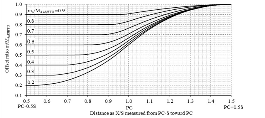 (a)
(a)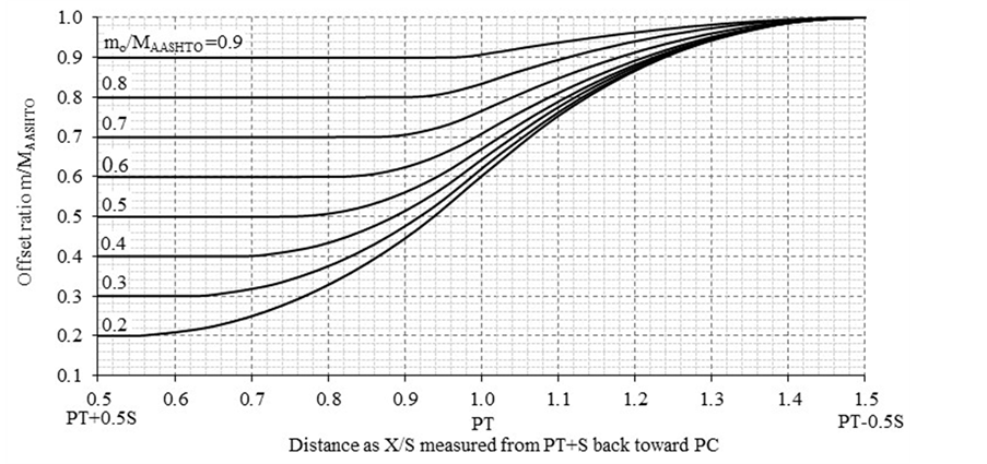 (b)
(b)
Figure 9. Chart of offsets to elliptical envelopes, L ≥ S and R/S = 2; (a) For segments from PC − 0.5S to PC + 0.5S; (b) For segments from PT + 0.5S back to PT − 0.5S.

Figure 10.Chart of offsets to elliptical envelopes for segments from PT − 0.5S to PT + 0.5S, L ≥ S, R/S = 2.
9. Summary and Conclusions
This paper presents analysis of innovative use of Euler’s spiral as minimum roadside clearance envelope. The analysis compares available sight distances provided by the innovative envelope and those provided by the envelope resulting from use of clearance offsets developed by Raymond [2] . Raymond’s offsets are used as basis of comparison since the offsets are accurate, have been recommended in the green book, and implemented in the field for more than 40 years. For both the innovative envelope and Raymond’s envelope available sight distances were determined with only a subject vehicle on the road and no vehicle downstream of the subject vehicle. That setting guarantees that available sight distances are a function of roadway and roadside geometry only and not a function of space headways.
Results of comparison revealed that clearance offsets determined with the innovative envelope are greater than minimum offsets determined with Raymond’s model. Therefore, the innovative envelope may be used for clearance of roadsides especially on sites with either large radii and/or wide offsets to boundaries of clear zones on tangent sections. Quantitatively, the envelope will fit sites whose offsets to the boundaries of clear zones are equal to or greater than 67% of the offset determined with Equation (1), that is, sites with .
.
On sites with either short radii and/or narrow clear zones on tangent sections (i.e. ), there is no need of clearing sections near PC − 0.5S since available offsets (to clear zone boundaries) already provide sight distances that are longer than stopping sight distances. Moreover, the long offsets near PC − 0.5S will be unutilized fully because part of the cleared area does not accommodate sightlines, especially on sites with short tangent sections. Where highways pass through cut zones, it is advised to save money that could be used to clear areas that do not accommodate sightlines. Money could be saved through providing large radii or through providing transition from boundaries of clear zones on tangent sections to effective portions of the Euler’s spirals.
There are several curves that geometric designers can creatively use for roadside clearance envelope. A designer may choose any of them as long as the chosen curve has offsets that are greater than minimum values determined with either the graphical method, Raymond’s chart [2] , Glennon’s chart [3] , or Mauga’s chart [4] [5] . Also, the chosen curve should not have very long offsets that may result in extra earthwork costs where highways pass in cut zones. For example, elliptical arcs meet the two criteria as demonstrated in this paper. Advantages of elliptical arcs include their flexibility in aligning well with boundaries of clear zones on tangent sections regardless of radii of highway curves. To add, elliptical arcs can be used to consistently provide extra available sight distances within highway curves as on tangent sections without needing extra clearance on the tangent sections. In this paper, a sample design chart for offsets to elliptical clearance arcs has been presented. The offsets are minimum values needed to provide a given sight distance while gradually transitioning clearance from clear zone boundaries to AASHTO’s offset M.
Cite this paper
Mauga, T. (2017) Suitability of the Euler’s Spiral for Roadside Clearance in Order to Provide Stopping Sight Distances. Journal of Transportation Technologies, 7, 221-239. https://doi.org/10.4236/jtts.2017.73016
References
- 1. American Association of State Highways and Transportation Officials (AASHTO) (2011) A Policy on Geometric Design of Highways and Streets. AASHTO, Washington DC.
- 2. Raymond, W.L. (1972) Offsets to Sight Obstructions near the Ends of Horizontal Curves. ASCE Journal of Civil Engineering, 42, 71-72.
- 3. Glennon, J.C. (1987) Effects of Sight Distance on Highway Safety. Transportation Research Board (TRB) State of the Art Report No. 6, Washington DC, 64-77.
- 4. Mauga, T. (2014) Horizontal Clearance Offsets to Objects Higher than Sightlines. Transportation Research Record, 2436, 23-31.
https://doi.org/10.3141/2436-03 - 5. Mauga, T. (2015) New Spiral Curves for Appropriate Transition of Minimum Roadside Clearance on Simple Curves. Journal of Transportation Technologies, 5, 141-158.
https://doi.org/10.4236/jtts.2015.53014 - 6. Mauga, T., Ghanma, M. and Ahmed, K. (2013) Roadside Clearance Limit on Horizontal Curves with Transition Arcs. Transportation Research Record, 2358, 20-28.
https://doi.org/10.3141/2358-03 - 7. Mauga, T. (2016) Minimum Clearance Offsets for Providing Desired Sight Distances at Simple Curves with Variable Operating Speeds. Journal of Transportation Technologies, 6, 106-117.
https://doi.org/10.4236/jtts.2016.63010 - 8. Ameri, M., Rostami, T., Mansourian, A. and Salehabadi, E. (2012) New Method for Determination of Driver Sight Distance from Roadside Obstacles on Horizontal Curves. Journal of Basic and Applied Scientific Research, 2, 141-158.
- 9. You, Q.C. and Easa, S.M. (2016) Innovative Roadside Design Curve of Lateral Clearance: Roadway Simple Horizontal Curves. Journal of Transportation Engineering, 142.
https://doi.org/10.1061/(asce)te.1943-5436.0000889 - 10. American Association of State Highways and Transportation Officials (AASHTO) (2011) Roadside Design Guide. AASHTO, Washington DC.
- 11. Medina, A.M.F. and Tarko, A.P. (2004) Reconciling Speed Limits with Design Speeds. Report No. FHWA/IN/JTRP-2004/26, West Lafayette, IN.
- 12. Mauga, T. (2013) Extension of the AASHTO Model for Horizontal Sightline Offset to Apply to Beginnings and Ends of Simple Horizontal Curves. TRB Annual Meeting, Washington DC, Paper Numbers: 13-0558, 13-0558.