Agricultural Sciences
Vol.3 No.3(2012), Article ID:19030,8 pages DOI:10.4236/as.2012.33037
Sources of inaccuracy when estimating economically optimum N fertilizer rates
![]()
Technische Universität München, Center of Life Sciences Weihenstephan, Freising, Germany; bachmai@wzw-tum.de
Received 5 January 2012; revised 16 February 2012; accepted 12 March 2012
Keywords: Confidence Interval; Economic Optimum; N Rate Trials; Quadratic Model; Linear-plus-Plateau Model
ABSTRACT
Nitrogen rate trials are often performed to determine the economically optimum N application rate. For this purpose, the yield is modeled as a function of the N application. The regression analysis provides an estimate of the modeled function and thus also an estimate of the economic optimum, Nopt. Obtaining the accuracy of such estimates by confidence intervals for Nopt is subject to the model assumptions. The dependence of these assumptions is a further source of inaccuracy. The Nopt estimate also strongly depends on the N level design, i.e., the area on which the model is fitted. A small area around the supposed Nopt diminishes the dependence of the model assumptions, but prolongs the confidence interval. The investigations of the impact of the mentioned sources on the inaccuracy of the Nopt estimate rely on N rate trials on the experimental field Sieblerfeld (Bavaria). The models applied are the quadratic and the linear-plus-plateau yield regression model.
1. INTRODUCTION
The effect of N fertilizer on the yield of agricultural crops can be studied using N response functions. Such functions are usually fitted to the data from N rate trials by regression. The available function types used for modeling purposes in the course of this discussion are for example, quadratic (e.g. [1,2]) or the linear-plus-plateau functions (e.g. [3]) and the Mitscherlich, which is a kind of exponential model [4,5]. Other researchers had additionally investigated the quadratic-plus-plateau model [6,7], the square-root model [6,8] and even more complicated models [9]. On the basis of the assessed production functions, ex post analyses were carried out for the economically optimum N application.
The economic optimum is reached when the marginal cost of the N fertilization corresponds to the marginal revenue, i.e. when the returns above the N fertilizer cost (RANC) are maximized. For a given product price p (in EUR·Mg–1) and a N fertilizer price r (in EUR·kg–1), these returns are computed as
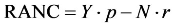 (1)
(1)
where Y is the measured yield in Mg∙ha–1 and N is the N rate in kg∙ha–1. The N rate where these returns above the N fertilizer cost are maximized, is the economically optimal N rate, Nopt.
The evaluation of any N rate trial is usually followed by the analysis of the residuals and the determination coefficient R2, to justify the choice of the model applied. However, as discovered by [6], R2 is not a suitable measure, as it barely depends on the model chosen. The point estimate for Nopt, which is derived from the fitted model does not however provide any information on the accuracy or reliability. Therefore, our objective is to compute and discuss confidence intervals for Nopt, which will be based on quadratic and linear-plus-plateau N response functions, with the consideration of extensive N rate trials as an example. The results could be used for optimizing decision making in nitrogen management. However, we shall see that the confidence intervals are very long, and further, they strongly depend on the model chosen and on the area of N levels used to fit the model using regression functions. These sources of inaccuracy make it nearly impossible to locate the optimum N fertilizer rate in a way that supports decision making.
2. METHODS OF ESTIMATING THE OPTIMUM N-APPLICATION RATE
2.1. Point Estimate and Confidence Set in the Quadratic Model
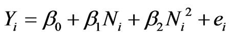
In the quadratic yield model, the expected yields, E(Yi), are described by a quadratic function of the total N application rates, Ni. Therefore, the yields, Yi, i = 1, ∙∙∙, n, were modeled as random variables that depended on Ni in the following way:
 (2)
(2)
Ni denote fixed levels of N application rates, bj, j = 0, 1, 2, the fixed unknown coefficients of regression, and ei the error variables, which are assumed to be independent and normally distributed with an expected value 0 and a common unknown variance s2 > 0. The unknown coefficients bj, are estimated using the least-squares estimates bj. This requires at least three different N-levels. Otherwise the estimates would not be unique.
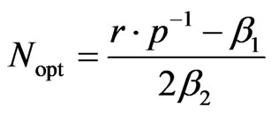
The economically optimal N application rate, Nopt, is the N-rate where the expected returns above N fertilizer cost, E(RANC) = p×(b0 + b1N + b2N2) – r×N, are maximized. This applies to the following optimum N rate:
 (3)
(3)
Nopt results from the N where the first derivative of the model parabola, E(Y) = b0 + b1N + b2N2, equals r×p–1, which is the ratio between N fertilizer and the product price.
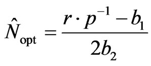
By using the least-squares estimates bj for estimating the coefficients bj, the point estimate for Nopt was immediately reached :
 (4)
(4)
Note that this point estimator, is biased1 because it is not a linear combination of the unbiased least-squares estimators b1 and b2. It is in essence a ratio.
According to [10]’s duality with confidence intervals and tests, a confidence interval or, more generally, a confidence set for Nopt consists of all hypothetical values N0 whose simple null hypothesis,
 , (5)
, (5)
cannot be rejected. By using (3), the null hypothesis in (5) can be reshaped to
 . (6)
. (6)
This is a linear hypothesis, so it can be tested in the framework of general linear models using the usual Ftest [11], which is a likelihood ratio test. Therefore, the corresponding confidence set is called a likelihood interval, provided that it is an interval. This usually applies but it does not need to. As mentioned before, it is formed by the set of all N0 for which H0 in (5) or (6) cannot be rejected. For those interested in the area of statistical inference, this test and the corresponding derivation of the confidence set, which can be produced by explicit mathematical formulae, is described fully in [12]. The computation of this likelihood-type confidence set for Nopt was implemented in the Fortran program VINO. EXE, which can be downloaded from the internet [13]. It is analogous to that of [14], who calculated it for the ratio of parameters, and to that of [15], who computed it for the maximum of a quadratic regression.
Under the assumptions made (quadratic model, independent and normally distributed homoscedastic errors), tests of linear hypotheses, such as in (6), are considered exact, so exact confidence intervals are obtained, whereas confidence intervals derived according to [11,16,17], which are also called Wald intervals, would only provide approximate confidence intervals. They are symmetric around the point estimate, which is not even unbiased. Therefore, they “may not accurately reflect the actual, often asymmetric, uncertainty in an estimate” [18]. Such an asymmetric situation is given here as seen with rapidly increasing fertilizer application rates. The true yield function decreases more slowly, as indicated by the quadratic model, which overestimates the yield loss due to lodging [19]. Therefore, the Delta method will not be pursued but the likelihood intervals will be used to proceed exactly as mentioned above. These intervals are not symmetric around the point estimate, so neither limit depends on the other and they can adapt better to the data around either limit. The lower limit of the confidence interval is in the focus of ecological interests as it gives the minimum fertilization that cannot be rejected as being optimal.
2.2. Point Estimate and Confidence Set in the Linear-plus-Plateau Model
In the linear-plus-plateau model, the economic optimum, Nopt, equals the transition of the increasing straight line to the horizontal, unless the price ratio rp–1 is greater than the gradient of the increasing straight line (cf. [20]), which, however, usually not applies. The mentioned transition to the horizontal is a parameter of the linearplus-plateau model. The program PRISM not only estimates the model parameters, but also calculates approximate confidence intervals for them [21]. Therefore, point estimates and confidence intervals for Nopt could be obtained using PRISM. They do not, contrary to the parabola-based confidence sets, depend on prices.
3. THE FIELD SITE
The test field, Sieblerfeld (5 ha), is in the Tertiary hills of Upper Bavaria, Germany, and it has two very different yield zones. The soil texture in the high yielding-zone is a sandy loam with an available field capacity of the rooted soil horizons of 160 mm. In the low-yielding zone the soil texture is a loamy sand with an available field capacity of the rooted soil horizons of 100 mm [22]. Within the two distinct yield zones, N-rate test areas were designated to derive site-specific N-response functions. For this, N-rate trials were carried out in the season 2001/02 on winter wheat (Triticum aestivum L.).
The trial design was a randomized complete block design with four blocks in each yield zone. To investigate the dependence between yield and N fertilizer rate, 11 plots that were given with different rates of N (0, 80, 100, 120, 140, 160, 180, 200, 220, 240 and 260 kg∙ha–1) were selected randomly from each block in both zones, so that there were n = 44 yield measurements in each yield zone. The yields were measured with a plot combine. The plots were 12.5 m2 with a length of 10 m and a width of 1.25 m. Figure 1 illustrates the randomization results at the midpoints of the plots; these were recorded with a precision of 1 m with GPS technology.
Note that randomized complete block designs are advantageous over complete block strip trials because only the former ensures independence of the variable under study. Designs of the latter kind are widely used [23-25],
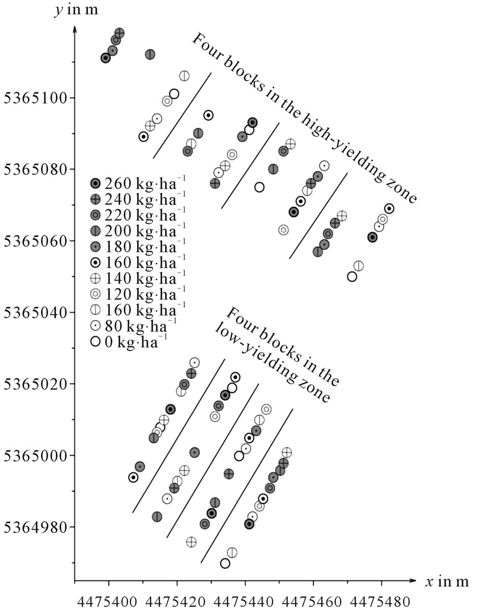
Figure 1. The randomized complete block design represented by the measured Gauss-Krüger coordinates x and y of the plot mid points.
but their lack of randomization within strips can result in the type of strip heteroscedasticity and correlation identified in [19]. In particular, correlations within strips occur in monitored yield data [1,25,26] because of the threshing system’s mass flow and the yield monitor’s datapreprocessor.
4. RESULTS AND DISCUSSION
The results are presented in four figures (Figures 2-5) with different models and different designs of N levels. The narrow boxes show the confidence intervals, or, more generally, the confidence sets for Nopt when the ratio between N fertilizer price r and crop price p is r×p–1 = 0.0054545 (EUR·kg–1) (EUR·Mg–1)–1 = 5.4545. This applies, for example, to r = 1.20 EUR·kg–1 and p = 220 EUR·Mg–1. This ratio corresponds to the model’s target slope that is to be reached by the optimum N fertilization. It is indicated by dotted lines.
4.1. Assumption Check
In [27] where the same trial was evaluated to test the precision agriculture hypothesis (no difference between the optimum N-rate in highand low-yielding zone) and to compute confidence intervals for the difference of the N optima, the usual assumptions have been checked. The result was that the data can be assumed to be approximately normally distributed and homoscedastic, and further, a block effect in the randomized complete block design could not be detected, although the N rate trials were very extensive. Therefore, the ordinary regression

Figure 2. All measured values (including the zero N rate), regression curves and confidence sets for Nopt in both yield zones of the Sieblerfeld trials, where the ratio between N fertilizer price r and crop price p is r×p–1 = 5.4545, e.g. r = 1.20 EUR·kg–1 and p = 220 EUR·Mg–1.
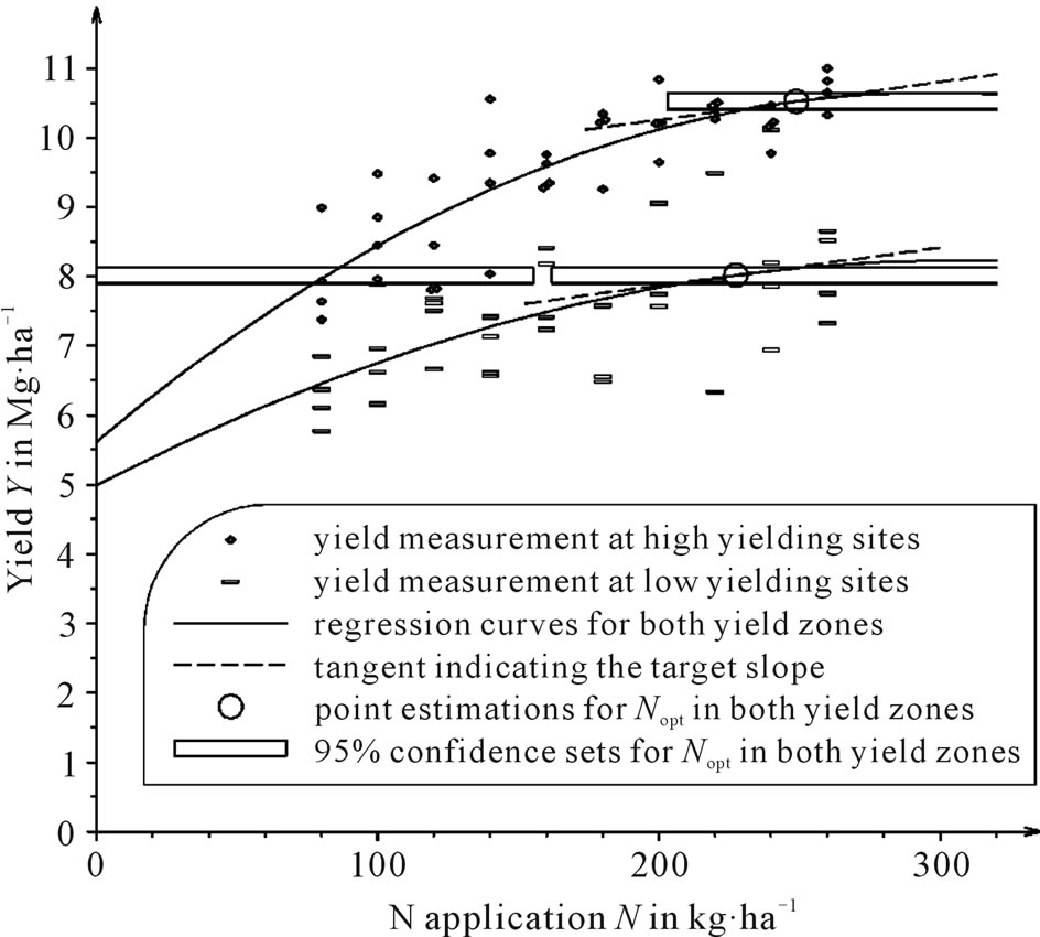
Figure 3. All measured values except the zero N rate, regression curves and confidence sets for Nopt in both yield zones of the Sieblerfeld trials, where the ratio between N fertilizer price r and crop price p is r×p–1 = 5.4545, e.g. r = 1.20 EUR·kg–1 and p = 220 EUR·Mg–1.
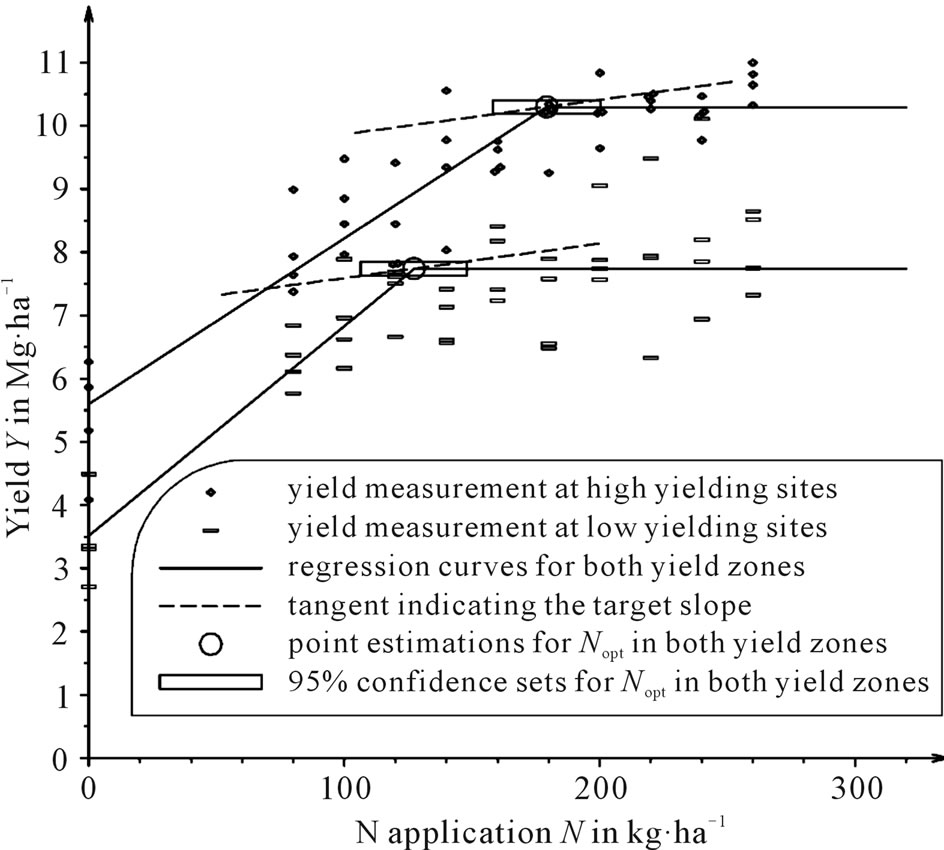
Figure 4. All measured values (including the zero N rate) as fitted by the linear-plus-plateau model and confidence sets for Nopt in both yield zones of the Sieblerfeld trials, where the ratio between N fertilizer price r and crop price p is r×p–1 = 5.4545, e.g. r = 1.20 EUR·kg–1 and p = 220 EUR·Mg–1.
analysis and the mentioned methods to compute confidence sets for the N optima, can be applied.
4.2. The Assymmetry of the Confidence Intervals in the Quadratic Model
A likelihood ratio confidence interval in the quadratic model need not be symmetric around the point estimate. In Figure 2 for example, where the design of all N levels
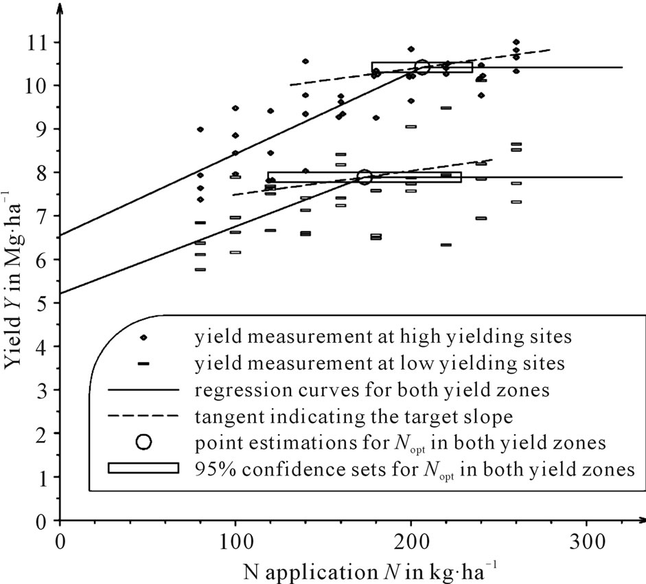
Figure 5. All measured values except the zero N rate as fitted by the linear-plus-plateau model and confidence sets for Nopt in both yield zones of the Sieblerfeld trials, where the ratio between N fertilizer price r and crop price p is r×p–1 = 5.4545, e.g. r = 1.20 EUR·kg–1 and p = 220 EUR·Mg–1.
including the zero N rate is considered, the confidence interval [204 kg∙ha–1, 328 kg∙ha–1] for the high-yielding zone is only 36 kg∙ha–1 long to the left of the point estimation 204 kg∙ha–1, whereas to the right it is 88 kg∙ha–1, which is nearly three times as long. This is, above all, due to the fact that yields from very high N rates do not seem to sink. For the low-yielding zone, a point estimation of 199 kg∙ha–1 and a confidence interval of [173 kg∙ha–1, 260 kg∙ha–1] present a similar situation with regards to the asymmetry. It seems that a concave parabola with a vertex at the far right of the point estimation is easily compatible with the measured data, whereas a concave parabola with a vertex at the far left of the point estimation is not suited for fitting the yields, since those to the right of such a vertex do not sink.
4.3. The Length of the Confidence Intervals
We can see in Figures 2-5 that all confidence intervals or, more generally, confidence sets are very long.
In Figure 2 for example, the 95% confidence interval for Nopt in the low-yielding zone [173 kg∙ha–1, 260 kg∙ ha–1], is somewhat shorter than the 95% confidence interval for Nopt in the high-yielding zone [204 kg∙ha–1, 328 kg∙ha–1]. This can be explained as follows. In contrast to the high-yielding zone, the higher N doses in the lowyielding zone did not result in further increases in yield while a small yield depression could even be observed at 260 kg∙ha–1 that forced the regression function to go down. Consequently, the parabola’s maximum can be more clearly determined so that a long confidence interval could also be avoided. Higher N rates in the higheryielding zone have a shortening effect on the confidence interval for Nopt.
When considering the enormous length of both the 95% confidence intervals, it becomes clear that even in such extensive N rate trials, the ex post estimated optimum N rates can only be roughly estimated. It is not possible, in retrospect, to limit the optimal nitrogen quantity to a level of less than 87 kg∙ha–1 length in the low-yielding zone or 124 kg∙ha–1 in the high-yielding zone. The length of the confidence intervals results from the fact that N fertilization have a very wide marginal profit area. From the economic point of view, however, the additional N quantity used ruins the economic advantage of the increase in yield. This leads to a very flat function around the optimum for returns above N fertileizer cost, making it compatible with many model parabolae with widely ranging vertices. The set of these vertices is the confidence interval, which is therefore very long.
The length of the confidence intervals gives us a first insight into the uncertainty concerning the true, unknown Nopt. Although their enormous length makes clear that reasonable statements about Nopt can hardly be made, this source of uncertainty is the only one that can be controlled statistically because the confidence sets could be shortened if more data were available.
4.4. The Influence of the N Rate Trial Design on the Confidence Sets
In order to analyze the influence of the N rate trial design on the point estimate and confidence set for the economically optimum N rate, point estimates and confidence intervals for Nopt with different designs of N levels were calculated. In Figure 2 and Figure 4, all N levels (0, 80, 100, 120, 140, 160, 180, 200, 220, 240 and 260 kg∙ha–1) are considered, whereas in Figure 3 and Figure 5 the zero N rate is disregarded.
Taking zero fertilization not into account leads to a higher estimation of the economically optimum N rate, Nopt, and to the lengthening of the confidence interval. This can be observed in the quadratic model (compare Figure 3 to Figure 2) as well as in the linear-plus-plateau model (compare Figure 5 to Figure 4). In the lowyielding zone, the 95% likelihood confidence set based on the quadratic model (Figure 3) is no longer an interval. It is made up of all real numbers with the exception of an interval. The reason for such degenerated confidence sets is that the shape of the parabola, concave or convex, around which the data disperse, cannot be clearly recognized when the zero N rate is omitted. The data could be fitted passably by a line with a positive gradient and thus, almost equally, by very wide parabolae whose vertices lie to the far left if they are convex and to the far right if they are concave. In this way, a gap-type confidence set arises, which contains N-coordinates for profit maxima (on the right of the gap) as well as profit minima (on the left of the gap).
The gap could disappear if, in addition, the error probability were so “little” that every vertex can be considered as being a “little” compatible with the data. In practice, all these confidence sets are, of course, worthless. Based on the research findings, feasible fertilization rules cannot be given at a high level of confidence. The gap type or the extreme length of these confidence sets, without zero fertilization, is an indication of the fact that the function for the returns above N fertilizer cost, which is to be maximized, must be relatively flat in the area of its maximum, making it very difficult to locate.
If, however, the zero N rate is taken into account (Figure 2), the parabola is forced to sink as a result of the low yield under no fertilization, but not just to the left of the maximum: The symmetry of the parabola means that it would sink to the right as well. In this way, the region around the maximum is less flatly modeled as it appears to be in reality. The shorter length of the confidence interval that results from this may also possibly be attributed to a weakness in the quadratic model in the area of N optimum.
However, by excluding zero fertilization, the model is limited to a really small area of interest and the weakness is then of little importance. The smaller the region, the better it can be modeled by a simple function. On the one hand, the confidence interval is extended when omitting the zero fertilization, but on the other hand, it is also made more trustworthy since it is less influenced by the model assumptions.
4.5. Comparison of Confidence Sets with Respect to the Underlying Model
In the introduction five function types used for modeling the yield response are mentioned (quadratic, linearplus-plateau, Mitscherlich, quadratic-plus-plateau, squareroot). The evaluation of N rate trials based on these models is related to the point estimates for Nopt. Usually, confidence intervals are only computed in the linearplus-plateau model, where Nopt is one of its parameter. The confidence intervals of [2], however, are also based on the quadratic model, but they were not compared with those based on the linear-plus-plateau model. Yet we shall see that such a comparison, which shall be made in the following, reveals large differences.
As far as the goodness of fit is concerned, it can be stated that both models, the quadratic (Figure 2 and Figure 3) and the linear-plus-plateau model (Figure 4 and Figure 5), fitted equally good. Reference [6] also made the same conclusion, but this does not validate the finding completely because, despite this similarity, [6] and many other authors found marked discrepancies with respect to the Nopt (cf. [28-31]).
Such discrepancies also apply to the confidence intervals for Nopt and their length. The linear-plus-plateau model provides smaller confidence sets. When considering all N levels, as in Figure 4, the increasing straight line’s slope is 0.026 (Mg∙ha–1) (kg∙ha–1)–1 = 26 for the high-yielding zone and 0.033 (Mg∙ha–1) (kg∙ha–1)–1 = 33 for the low-yielding zone. Figure 5 depicts the design without the zero N rate, where the slope of the increasing straight line of the linear-plus-plateau model is 19 for the highand 15 for the low-yielding zone. All these slopes are greater than the realistic price ratios rp–1. Thus, the economic optimum, Nopt, equals the transition of the increasing straight line to the horizontal, where confidence intervals for Nopt could be obtained using PRISM [17].
The shorter length of the confidence intervals can be attributed to the fact that the transition from the increaseing straight line to the horizontal is clearly easier to identify than the position where a parabola has a rather flat positive gradient (Figure 2 and Figure 3). It is not surprising that the inferences from the two models, the linear-plus-plateau and the quadratic one, which are based on such very different biological assumptions, are incompatible. Nevertheless, it may be surprising that the confidence intervals for Nopt differed so much in both models. When considering only the design with all N levels, these confidence intervals did not even overlap. In the high-yielding area, the linear-plus-plateau model resulted in a 95 % confidence interval of [158 kg∙ha–1, 200 kg∙ha–1] (Figure 4), whereas the quadratic model yielded a confidence interval of [204 kg∙ha–1, 328 kg∙ha–1] (Figure 2). The same pattern was seen in the low-yielding area: If the linear-plus-plateau Model is assumed to be true, then the Nopt estimate lies between 106 and 148 kg∙ ha–1 (Figure 4), whereas the quadratic model considers fertilization between 173 and 260 kg∙ha–1 (Figure 2) as optimal.
The latter clearly shows that a confidence interval does not sufficiently enough reflect the uncertainty of the true optimum N rate. The fact that the true exact model is unknown and that no simple model reflects the reality in an appropriate way makes the uncertainty much greater.
5. CONCLUSIONS
From statistical point of view, the accuracy of the Nopt estimate can be seen from a confidence interval. Confidence intervals would become shorter if the trials were based on more data. Their length would even tend to zero if the number of data tended to infinity, and thus, it seems that the inaccuracy of the Nopt estimate could be controlled by expanding the field trials.
However, as the Sieblerfeld trials have shown, another source of inaccuracy of the Nopt estimate is given by the yield response model, because no model reflects reality exactly. As far as the point estimation of Nopt is concerned, marked discrepancies with respect to the underlying model had already been pointed out by many authors [6,28-30]. These discrepancies equally affect the corresponding confidence intervals, and therefore, the confidence sets differ with respect to the model choice. In the Sieblerfeld trials, confidence intervals could be obtained that did not even overlap when computed on the basis of two different models (quadratic and linear-plus plateau). This kind of uncertainty would not decrease by expanding the trials.
A third source of inaccuracy arises from the chosen design of N levels on which the model is fitted. To avoid long confidence intervals or even gap-type confidence sets, which additionally contain profit minima, the empirical data should clearly indicate a concave model, and therefore, the confidence intervals should be based only on designs that include the zero N rate and very high N. By using such datasets, these extreme N levels will have, due to their leverage effect, a strong influence on the regression function and thus also on the point estimation and the confidence interval for Nopt. These are then mainly determined by the choice of the modeling of the yield function between the extreme N levels, which lie far away from the economic optimum. Therefore, to diminish the large impact of the model choice on the Nopt estimate, the area on which to fit the model should only be a small neighborhood around the supposed true N optimum. Then, however, a concave shape of the N-Y scatterplot is no longer clearly indicated, and large confidence sets would arise. They would be more trustworthy as they less depend on the model choice, but to make them usable, they need to be much smaller, which requires an exorbitant increase of the number of data in the trial, and this is hardly possible in practice.
The wide range and large difference of confidence intervals under different models and N level designs might also be attributed to the fact that the area of N fertilizer applications that are very close to the economic optimum is very wide. It is a general experience that the economic profit would not reveal much of a difference in an N application range of 150 kg∙ha–1 to 250 kg∙ha–1. Usually, each of these values lies in approximation to the optimum. From an ecological point of view, the challenge should be to identify the corresponding N rate recommendations on the basis of trial results from the lower limit of such ranges, so that economically unnecessary N balance surpluses are avoided.
REFERENCES
- Lambert, D., Lowenberg-DeBoer, J. and Bongiovanni, R. (2002) Spatial Regression, an alternative statistical analysis for landscape scale on-farm trials: Case study of variable rate nitrogen application in Argentina. Proceedings of the 6th International Conference on Precision Agriculture, ASA/CSSA/SSSA, Madison.
- Hernandez, J.A. and Mulla, D.J. (2008) Estimating Uncertainty of economically optimum fertilizer rates. Agronomy Journal, 100, 1221-1229. doi:10.2134/agronj2007.0273
- Wagner, P. (1999) Produktionsfunktionen und Precision Farming (Response functions in the context of Precision Farming). Zukunftsorientierte Betriebswirtschaft und Informationstechnologien in der Agrarwirtschaft. Gießener Schriften zur Agrarund Ernährungswirtschaft, 29, 39- 66.
- Lark, R.M. and Wheeler, H.C. (2003) A method to investigate within-field variation of the response of combinable crops to an input. Agronomy Journal, 95, 1093-1104. doi:10.2134/agronj2003.1093
- National Academy of Sciences, National Research Council (1961) Statistical methods of research in economic and agronomic aspects of fertilizer response and use. Committee on economics of fertilizer use of the agricultural board, NAS-NRC Pub. 918, NAS-NRC, Washington DC.
- Cerrato, M.E. and Blackmer, A.M. (1990) Comparison of models for describing corn yield response to nitrogen fertilizer. Agronomy Journal, 82, 138-143. doi:10.2134/agronj1990.00021962008200010030x
- Bullock, D.G. and Bullock, D.S. (1986) Quadratic and quadratic-plus-plateau models for predicting optimal nitrogen rate of corn: A comparison. Agronomy Journal, 86, 191-195. doi:10.2134/agronj1994.00021962008600010033x
- Le Bail, M., Jeuffroy, M.-H., Bouchard, C. and Barbottin, A. (2005) Is it possible to forecast the grain quality and yield of different varieties of winter wheat from Minolta SPAD meter measurements? European Journal of Agronomy, 23, 379-391. doi:10.1016/j.eja.2005.02.003
- Colwell, J.D. (1994) Estimating fertilizer requirements: A quantitative approach. CAB International, Wallingford.
- Lehmann, E.L. (1986) Testing statistical hypothesis. John Wiley & Sons, Inc., New York.
- Weisberg, S. (2005) Applied linear regression. John Wiley & Sons, Inc., New York. doi:10.1002/0471704091
- Bachmaier, M. (2009) A confidence set for that x-Coordinate where the quadratic regression model has a given gradient. Statistical Papers, 50, 649-660. doi:10.1007/s00362-007-0104-1
- Bachmaier, M. (2011) Fortran programs: 1. Confidence set for the economically optimum nitrogen fertilization in the quadratic model: VINO.EXE. 2. Confidence set for that x-coordinate where the quadratic regression model has a given gradient (incl. special case: confidence set for the x-coordinate of the parabola’s vertex): CIGIGRAD. EXE and CIVERTEX.EXE. http://www.tec.wzw.tum.de/index.php?id=46&L=1
- Fieller, E.C. (1954) Some problems in interval estimation. Journal of the Royal Statistical Society, B16, 175-185.
- Koziol, D. and Zielinski, W. (2003) Comparison of confidence intervals for maximum of a quadratic regression function. Biometrical Letters, 40, 57-64.
- Mittelhammer, R.C., Judge, G.G. and Miller, D.J. (2000) Econometric foundations. Cambridge University Press, Cambridge, 183-185.
- Casella, G. and Berger, R.L. (2002) Statistical inference. Duxbury Press, Belmont.
- Cook, R.D. and Weisberg, S. (1990) Confidence curves in nonlinear regression. Journal of the American Statistical Association, 85, 544-551. doi:10.2307/2289796
- Boyd, D.A., Yuen, L.T.K. and Needham, P. (1976) Nitrogen requirement of cereals. Journal of Agricultural Science, 87, 149-162. doi:10.1017/S0021859600026708
- Waugh, D.L., Cate, R.B. and Nelson, L.A. (1973) Discontinuous models for rapid correlations, interpretation und utilization of soil analysis and fertilizer response data. International Soil Fertility Evaluation and Improvement Program, North Carolina Sate University, Raleigh.
- Motulsky, H.J. and Christopoulos, A. (2003) PRISM, Version 4.0. Fitting models to biological data using linear and nonlinear regression. A practical guide to curve fitting, GraphPad Software Inc., San Diego.
- Liebler, J. (2003) Feldspektroskopische messungen zur ermittlung des stickstoffstatus von winterweizen und mais auf heterogenen schlägen. Herbert Utz Verlag, Munich.
- Hurley, T.M., Malzer, G.L. and Kilian, B. (2004) Estimating site-specific nitrogen crop response functions: A conceptual framework and geostatistical model. Agronomy Journal, 96, 1331-1343. doi:10.2134/agronj2004.1331
- Hurley, T.M., Oishi, K. and Malzer, G.L. (2005) Estimating the potential value of variable rate nitrogen applications: A comparison of spatial econometric and geostatistical models. Journal of Agricultural and Resource Economics, 30, 231-249.
- Anselin, L., Bongiovanni, R. and Lowenberg-DeBoer, J. (2004) A spatial economic approach to the economics of site-specific nitrogen management in corn production. American Journal of Agricultural Economics, 86, 675- 687. doi:10.1111/j.0002-9092.2004.00610.x
- Bullock, D.S., Lowenberg-DeBoer, J. and Swinton, S.M. (2002) Adding value to spatially managed inputs by understanding site-specific yield response. Agricultural Economics, 27, 233-245. doi:10.1111/j.1574-0862.2002.tb00119.x
- Bachmaier, M. and Gandorfer, M. (2009) A conceptual framework for judging the precision agriculture hypothesis with regard to site-specific nitrogen fertilization. Precision Agriculture, 10, 95-110. doi:10.1007/s11119-008-9069-x
- Abraham, T.P. and Rao, V.Y. (1965) An investigation on functional models for fertilizer response studies. Journal of the Indian Society of Agricultural Statistics, 18, 45-61.
- Anderson, R.L. and Nelson, L.A. (1975) A family of models involving intersecting straight lines and concomitant experimental designs useful in evaluating response to fertilizer nutrients. Biometrics, 31, 303-318. doi:10.2307/2529422
- Barreto, H.J. and Westermann, R.L. (1987) YIELDFIT: A computer program for determining economic fertilization rates. Journal of Agronomical Education, 16, 11-14.
- Nelson, L.A., Voss, R.D. and Pesek, J.T. (1985) Agronomic and statistical evaluation of fertilizer response. In: Engelstad, O.P., Ed., Fertilizer Technology and Use, ASA, Madison, 53-90.
NOTES
1To see the biasedness, assume for simplicity that r = 0 and E(b1) = (1 = 1 and E(b2) = (2 = –0.5, so that the ratio of the expected values in (4) is equal to 1. Assume further that the variance of b1 is negligible, so that b1 ≈ 1, and consider the following two b2-values: b2 = –0.1 and b2 = –0.9, which are symmetric when (2 = –0.5. In the former case, the ratio in (4) is around 5, in the latter case around 0.56. The mean of both values is 2.78. If b2 is additionally assumed to be always negative, it is felt that the expected ratio in (4) is greater than Nopt, which results, according to (3), in the value 1.