Journal of Data Analysis and Information Processing
Vol.2 No.3(2014), Article
ID:49340,10
pages
DOI:10.4236/jdaip.2014.23009
Combinations of Feature Descriptors for Texture Image Classification
Alexander Barley, Christopher Town
University of Cambridge Computer Laboratory, Cambridge, UK
Email: alex.barley@cantab.net, cpt23@cam.ac.uk
Copyright © 2014 by authors and Scientific Research Publishing Inc.
This work is licensed under the Creative Commons Attribution International License (CC BY).
http://creativecommons.org/licenses/by/4.0/


Received 15 June 2014; revised 17 July 2014; accepted 4 August 2014
ABSTRACT
Texture recognition and classification is a widely applicable task in computer vision. A key stage in performing this task is feature extraction, which identifies sets of features that describe the visual texture of an image. Many descriptors can be used to perform texture classification; among the more common of these are the grey level co-occurrence matrix, Gabor wavelets, steerable pyramids and SIFT. We analyse and compare the effectiveness of these methods on the Brodatz, UIUCTex and KTH-TIPS texture image datasets. The efficacy of the descriptors is evaluated both in isolation and by combining several of them by means of machine learning approaches such as Bayesian networks, support vector machines, and nearest-neighbour approaches. We demonstrate that using a combination of features improves reliability over using a single feature type when multiple datasets are to be classified. We determine optimal combinations for each dataset and achieve high classification rates, demonstrating that relatively simple descriptors can be made to perform close to the very best published results. We also demonstrate the importance of selecting the optimal descriptor set and analysis techniques for a given dataset.
Keywords:Image Processing, Texture Analysis, Computer Vision, Image Classification
`
1. Introduction
Texture analysis remains a lively and challenging topic. There are many practical applications such as shape analysis, image segmentation, object recognition, image retrieval, texture synthesis, classification of biological and medical datasets, and aerial and satellite surveys. The goal of texture classification is to match a query image with a reference image or group such that the query has the same visual texture as the reference.
Visual texture is typically defined [1] as the statistical variation in position, size, shape and orientation of some visual features that are repetitive over an area. This may take the form of textons (basic repeating primitives) or quasi-periodic statistical features. Texture is a key property of any surface, and along with shading, stereo, contours and motion can be used to infer depth from a 2-dimensional image.
Much work has been done on creating advanced feature descriptors to improve the accuracy of texture classification systems, and there are many examples of successful approaches. In this paper we demonstrate that it is possible to achieve very good benchmark results using generic and well-established texture extraction techniques if they are correctly combined with an appropriate, modern machine learning approach. We apply several standard feature extraction techniques to the Brodatz, UIUCTex and KTH-TIPS datasets to perform a comparison study. We then combine them with a wide variety of machine learning approaches to determine the optimal combinations and therefore demonstrate that by carefully selecting the correct method, it is possible to achieve results that are close to more modern task-specific techniques.
2. Materials and Methods
2.1. Related Work
Texture classification is a widely studied problem. Although the implementation specifics naturally vary, most approaches typically requires similar stages:
• One or more texture descriptors are applied to the chosen dataset.
• An analysis is performed on the extracted features to derive a measure of similarity or distance between textures.
• The chosen metric is applied to the dataset to perform texture based image classification and evaluated relative to groundtruth.
Hossain and Serikawa [1] discuss a number of techniques for performing classification, including statistical and filtering based methods, but they do not discuss the relative performance of these techniques, or whether they are applicable to classification tasks.
Other studies, however, are commonly related to applying these features to new, specific data sets or applying new, more complex features to the standard datasets.
Gabor wavelets are still regularly applied to new tasks, including in the medical domain. Roslan and Jamil [2] use Gabor wavelets in texture segmentation for MRI data. This has a number of advantages over shape or colour based approaches, which are generally useful only in more specific circumstances. Reddy and Kumaravel [3] also used Gabor wavelets, along with various other wavelet techniques, to evaluate the quality of bone in Dental Computed Tomography images.
A large body of work also exists where comparison studies are performed on features with various datasets. Randen and Husøy [4] compare many basic feature extraction techniques over a range of segmentation and classification tasks including Gabor filter banks, Laws masks and eigenfilters. Sharma et al. [5] present a comparative study, applying auto-correlation, edge frequency, primitive-length, Law’s method and co-occurrence matrices to the Meastex dataset.
The datasets we examine are also often the subject of research with regards to new features and descriptors. Because the most significant information of a texture often appears in the occurrence of grain components, Kumar et al. [6] apply long linear patterns, bright features defined by morphological properties, to perform texture classification. They use arbitrarily chosen images from the Brodatz texture set for their tests. Sumama et al. [7] also analyse the Brodatz texture set and apply various Gaussian density curvelet and wavelet approaches to the texture recognition problem in the field of content-based image retrieval.
Zhang et al. [8] examine the Brodatz, UIUCTex and KTH-TIPS image datasets using a sparse keypoint method and a support vector machine (SVM) and find that the performance of their method exceeds commonly used techniques on many of these, and is equal on the others. Janney and Geers [9] also examine the Brodatz set, among others, using invariant features of local textures. Their method was superior to the state of the art at the time of publication, and performs at a lower computational cost.
The descriptors we study in this paper have also been applied to more recent datasets. Do et al. [10] use SIFT to perform classification on the Ponce dataset and report retrieval rates of up to 100% for various tasks. However, they do not perform a comparison with other features. Yang and Newsam [11] apply SIFT and Gabor features to land-use analysis of high resolution satellite imagery using an SVM and Maximum a Posteriori (MAP) approach. They perform comparisons between the features and their learning techniques, and find that SVM combines best with Gabor and MAP combines best with SIFT. SIFT is reported to be substantially faster, however.
Mustafa et al. [12] use the grey-level co-occurrence matrix (GLCM) to analyse Electroencephalography (EEG) images. Their approach produces a frequency representation of the EEG signal, and can use texture analysis in the form of the GLCM combined with Principal Components Analysis (PCA) on the resulting image to detect sleep disorder breathing.
Do and Vetterli [13] make use of the steerable pyramid features in their analysis applied to the VisTex dataset. Their paper discusses the general context of image retrieval. They perform classification using a hidden Markov model which demonstrates substantial improvement over existing attempts.
2.2. Image Datasets for Comparative Texture Analysis
The Brodatz texture set1 is probably the most widely used texture benchmark. The data set consists of 111 images extracted from the Brodatz texture album, which are each commonly subdivided into nine non-overlapping parts to produce a total of 999 images.
The UIUCTex dataset2 contains 25 texture classes with 40 images per class. This dataset has significant scale and viewpoint changes, and includes non-rigid deformations, illumination changes and viewpoint-dependent appearance variations. The UIUCTex dataset is the most challenging of the commonly used texture datasets due to its high intra-class variation.
KTH-TIPS3 is another challenging dataset for classification. There are ten texture classes, and each image is captured at nine scales spanning two octaves. Each is viewed under three illumination directions and three poses, giving a total of 81 images per material. There are 10 classes in this image set: aluminium foil, brown bread, corduroy, cotton, cracker, linen, orange peel, sandpaper, sponge and styrofoam producing a total of 810 images.
Some example images from each dataset are shown in Figure 1.
2.3. Grey-Level Co-Occurrence Matrix
The grey-level co-occurrence matrix [12] is a second-order statistical texture measure. The matrix is a relation between the intensities of neighbouring pixels: it stores the relative frequencies over an image with which varying intensities co-occur at a specific distance and orientation.
We use a window size of 1 at four orientations to generate the matrix. The image is iterated over, and for each pixel, we increase the value in the matrix representing the difference in intensity between itself and its neighbours to the right, below-right, below and below-left as shown in Figure 2. The feature set then consists of the angular second moment, the contrast, the entropy, the homogeneity, the mean and the variance calculated on the co-occurrence matrix.
2.4. Gabor Wavelets
Gabor wavelets [2] are filters consisting of a sinusoidal plane wave of some frequency and orientation mod-
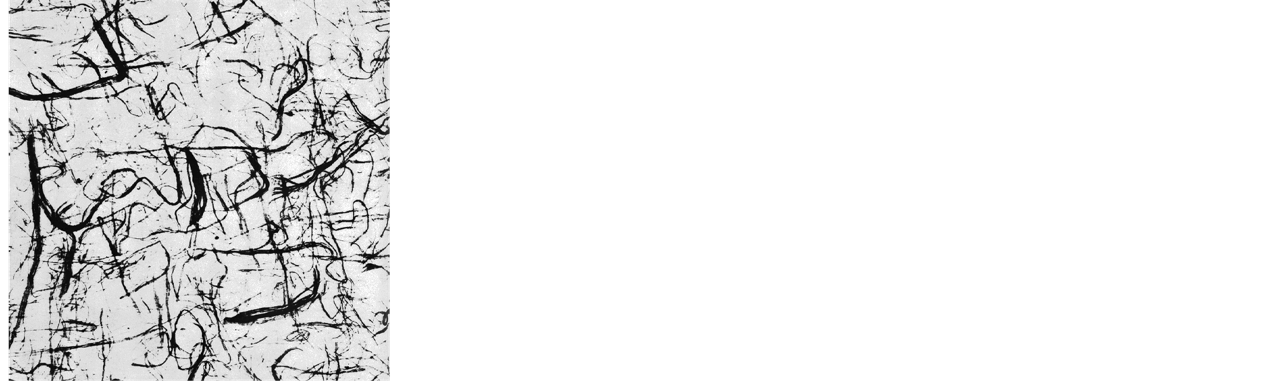

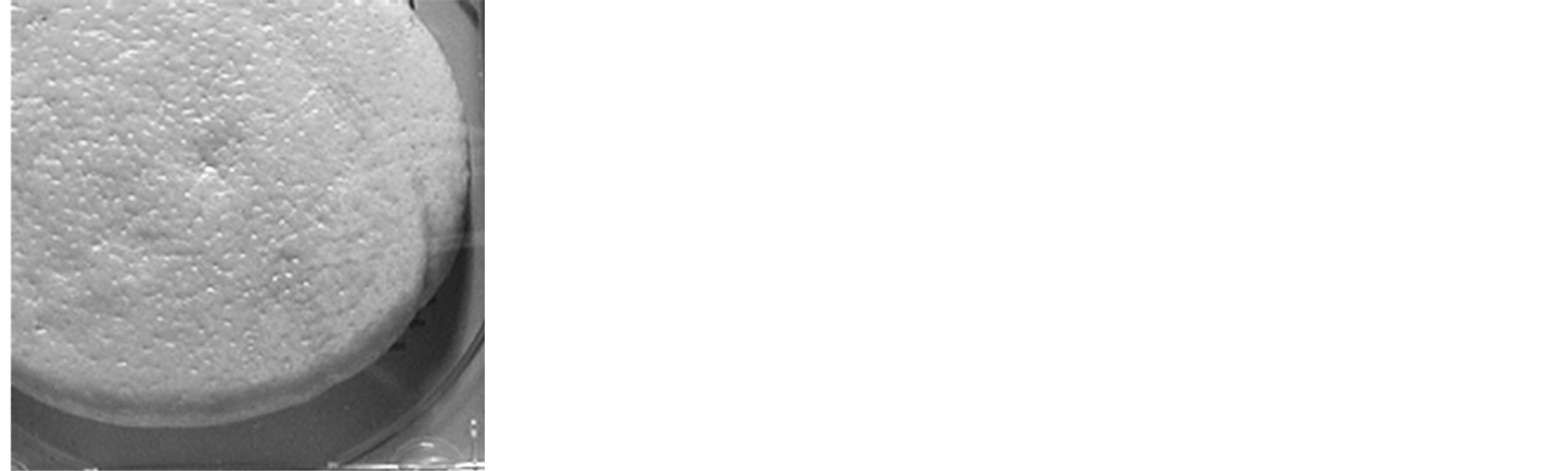
Figure 1. Sample images from the Brodatz, UIUCTex and KTH-TIPS datasets respectively.
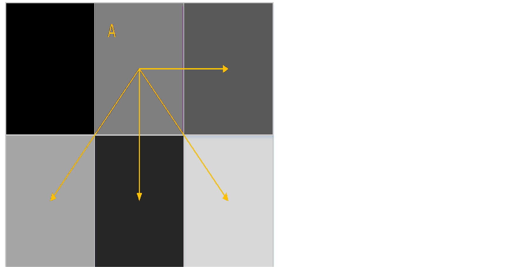
Figure 2. he neighbours of pixel A considered by the grey-level co-occurrence matrix when using four orientations and a window size of 1.
ulated by a Gaussian envelope. These band-pass filters allow the extraction of a single specific frequency subband: there will be a strong filter response when the frequency of the image in the specified orientation approximately matches the filter, and virtually no response if the orientation is wrong or the frequency is very different.
Gabor wavelets are particularly effective for image analysis because they uniquely minimise the joint uncertainty in the space and Fourier domains. Gabor wavelets can be generally considered as orientationand scaletunable edge and line detectors, and the statistics of these microfeatures are often used to characterise texture information.
Gabor wavelets are applied to texture classification through the use of a filter bank. We use a set of 24 wavelets with 6 orientations at 4 scales, as shown in Figure 3, each of which is convolved with the image to produce a feature response. We take the mean and standard deviation of the entire response to form a feature vector of length 48.
2.5. Steerable Pyramid
A pyramid representation of an image is formed of the original decomposed into sets of lowpass and bandpass components via Gaussian and Laplacian pyramids respectively [14] . A Gaussian pyramid can be formed by taking an image and repeatedly performing a Gaussian blur followed by subsampling. The Laplacian operator can be approximated by the difference between two Gaussians; by convolving a Gaussian with an image, fine detail in the image is removed. If the blurred image is then subtracted from the original, all that remains are the areas of fine details such as sharp edges. A Laplacian pyramid can therefore be generated by taking two consecutive levels in the Gaussian and taking the difference between them.
A steerable pyramid then applies a set of sinusoids to this scale-space pyramid by convolving with four oriented filters [15] :
 (1)
(1)
 (2)
(2)
 (3)
(3)
 (4)
(4)
The final stage of the steerable feature generation is creating the power maps, which represent the responses of the oriented filters at each scale. Taking the real and imaginary components of the 4 sinusoids yields 8 filters. To ensure the filter responses for each stage of the pyramid are equivalent, they must be reduced to the same scale. The same technique used to generate the Gaussian pyramid is therefore used to scale each filter result to the same size. The features for the steerable analysis are the average responses over the scaled power maps.
Figure 4 shows examples of the 24 power maps that are produced by the 8 filters being applied to 3 levels in the Laplacian pyramid. The technique used to extract features from the 24 maps is similar to that used for the Gabor wavelets. The mean of each power map and the standard deviation from the mean gives two features per map, meaning the final result of the analysis is a 48 element feature vector.
2.6. Scale Invariant Feature Transform
The Scale Invariant Feature Transform (SIFT) [16] transforms an image from pixel space into a set of keypoints. The goal of these features is to remain robust in the face of image scaling, rotation, and illumination. They should also remain consistent under noise. SIFT achieves this through scale-space extrema detection, keypoint localisation, orientation assignment and keypoint descriptor generation.
Formally, the scale space L of an image, is created by convolving the input image I with Gaussian filters G at different scales σ:

Neighbouring scales (σ and kσ for some constant k) are then subtracted from each other to produce the Difference-of-Gaussian images D:

Only scale-space extrema of D(x,y,σ) that have strong contrast are chosen as keypoints. This is done by computing the quadratic Taylor expansion of D(x,y,σ) around candidate keypoints
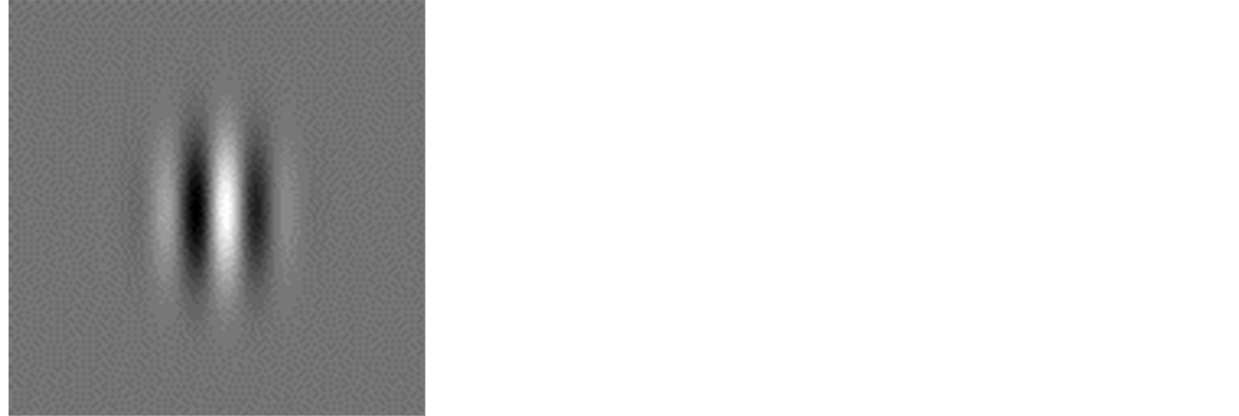
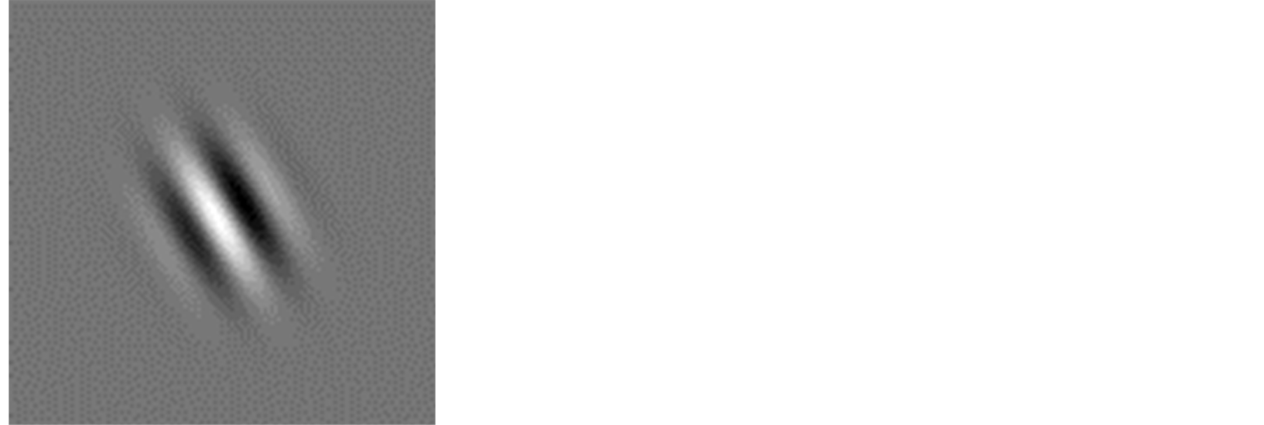

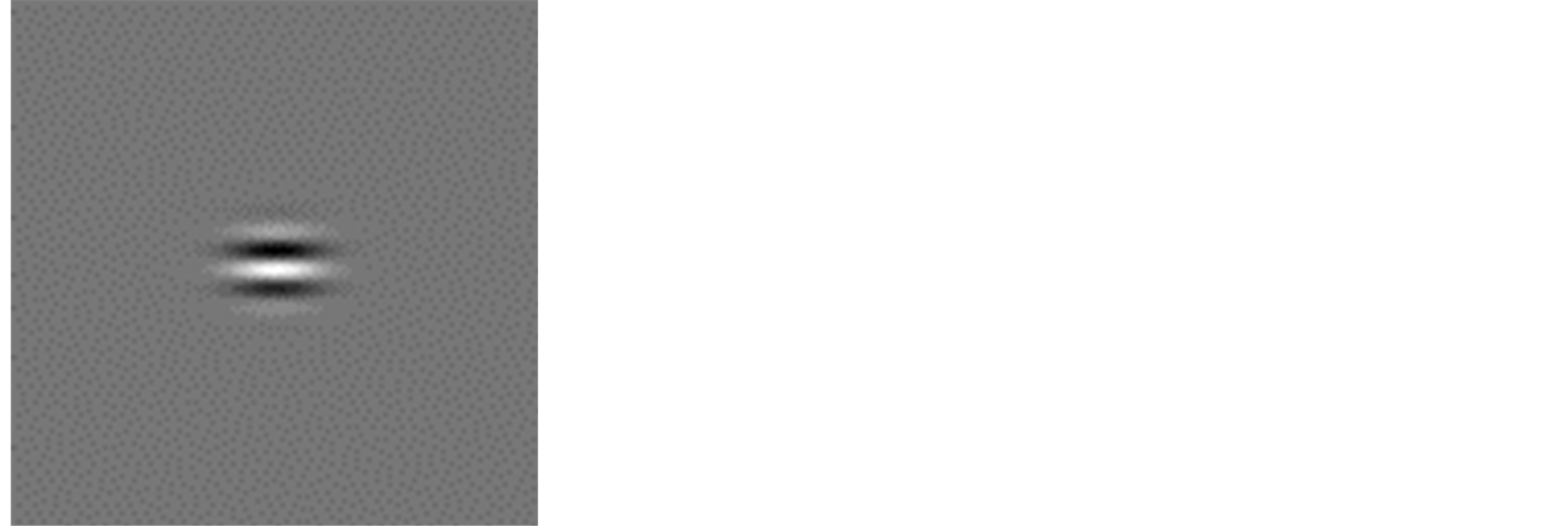
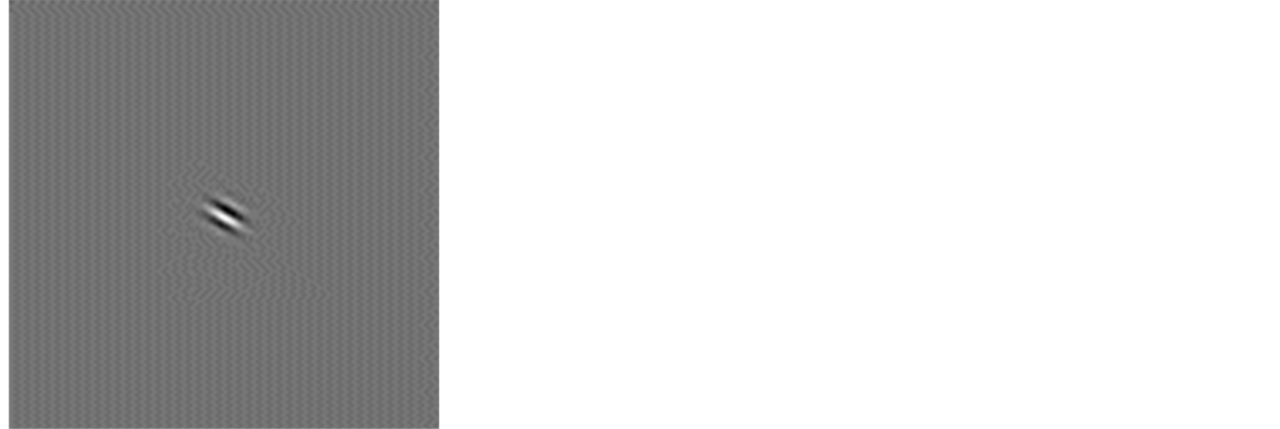

Figure 3. Samples of the Gabor wavelets at various scales and rotations that were used to perform texture feature extraction.
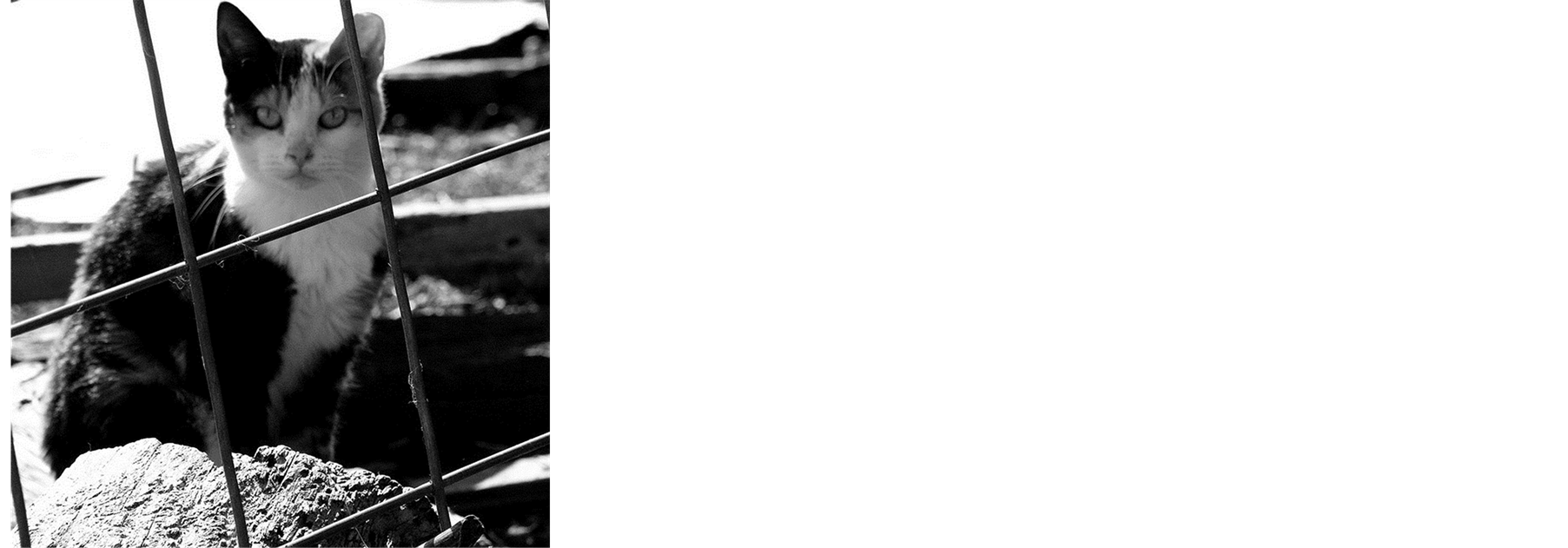
Figure 4. Example image (top) and samples of the 24 steerable power maps (inverted for clarity).

A keypoint descriptor based on local gradient directions and magnitudes is used. The descriptor is invariant to image rotations since the bins of the orientation histograms are normalised relative to the dominant gradient direction in the vicinity of the keypoint. The scale of analysis, and hence the size of the local region whose features are being represented, corresponds to the scale at which the given keypoint was found to be a stable extremum (subject to constraints on local contrast and contour membership).
2.7. Combination of Texture Descriptors
In addition to using features extracted using a single technique for classification, we also examine combinations of texture descriptors to determine whether this improves accuracy.
We define a feature combination as the concatenation of the feature vectors from two or more individual image feature extraction techniques.
In our analysis, we found that the increased number of features in the combinations would typically slow the machine learning stage significantly. For performance reasons, we therefore use Weka to perform an intermediate stage of principal components analysis on the new feature vectors prior to running the machine learning classifier.
The GLCM was excluded from the combinations due to its simplicity and poor optimal results. The combinations we performed were therefore:
• Steerable + Gabor
• Steerable + SIFT
• Gabor + SIFT
• Gabor + Steerable + SIFT The goal of performing these combinations is to determine whether the additional data provided by another machine learning technique can improve the classification performance of the system, if the results of the two techniques used individually are averaged, or if the additional data generally degrades performance below that of either technique used in isolation.
3. Results and Discussion
To evaluate the efficacy of the various texture descriptors, both in isolation and in combination, we present results on the challenging task of texture classification using the datasets described in Section 2.2.
To do so, we trained and evaluated classifiers using 10-fold cross validation. This technique randomly partitions the input data into 10 equally sized parts. 9 of these partitions are used for training, and the remaining set is used for testing. The process is then repeated a further 9 times such that each partition is used as the evaluation set exactly once. We used the following classifiers and utilised the default Weka settings:
1) Support Vector Machine (SVM)—a non-probabilistic binary linear classifier. The aim of a SVM is to form a hyperplane in high-dimensional space that can separate binary elements. It uses a kernel function to transform the data so that non-binary elements can be classified.
2) Bayesian network—a Bayesian classifier where the network is a probabilistic graphical model that represents a set of random variables and their conditional dependencies as a direct acyclic graph.
3) K-star—an instance-based learner that assigns instances to the most similar class based on the distance between them as described by an entropy based difference function.
4) IBk—an instance-based learner that applies K-nearest neighbours for any K.
5) Naive Bayes—a Bayesian classifier that makes the simplifying assumption that all features are independent.
6) Functional Tree (FTree)—a decision tree classifier that has logistic regression functions at the inner nodes to predict the value of a category-dependent variable based on predictor variables.
Table 1 shows the full results of the various datasets with each machine learning method. The best result we achieved for each dataset is marked in bold. We achieve an classification accuracies of up to 91.6% for the Brodatz dataset, 90.6% for the UIUCTex dataset and 96.2% for the KTH-TIPS dataset.
A comparison of the average and best success rates demonstrates the importance of selecting the correct machine learning technique for each classification task, as shown in Table2 There is an average improvement of 9.9% between the average accuracy rate of a feature over all classification attempts and the average accuracy of the same feature if considering only the best performing machine learning technique for each dataset.
The combined features, shown in Tables 3-5 only provide the optimal result for the UIUCTex dataset: when combining the steerable and SIFT features, an accuracy of 90.6% is achieved.
However, Table 6 shows that using feature combinations gives a better accuracy than using the individual texture features, with an average improvement of 6.13%, with a particularly significant improvement for the UIUCTex dataset. This suggests that in the case where the optimal combination of feature and machine-learning technique is not known, better accuracy will generally be achieved using a combination of features. This is likely due to the combination countering the weaknesses in any individual scheme.
Table 7 shows how the effectiveness of the various machine learning techniques changes when using the feature combinations as opposed to the individual features. The majority of machine learning techniques offer better average accuracy over all datasets using feature combinations.

Table 1. The accuracy percentages, before any optimisation, for the various combinations of texture set and analysis type. The best result for each texture set is marked in bold.
Table 2. Comparison of the average and best success rate for texture feature extraction techniques when considering all attempts, but excluding feature combinations.
Table 3. Results for the Brodatz texture set using combinations of features. The best overall result is marked in bold.
Table 4. Results for the UIUCTex texture set using combinations of features. The best overall result is marked in bold.
Table 5. Results for the KTH-TIPS texture set using combinations of features. The best overall result is marked in bold.
Table 6. Comparison of the average accuracy over each data set when using individual features or feature combinations.
Table 7. The average accuracy of each machine learning technique over all datasets when using the individual features or feature combinations.
Our results show that using feature combinations improves the average classification accuracy when a system cannot be tuned to an individual dataset or machine learning technique. If a specific machine learning technique is selected, feature combinations will typically perform better over a range of datasets, and the same is true if a specific dataset is selected and multiple machine learning techniques are used. Furthermore, when analysing a specific dataset using a specific machine learning technique, the range of results in feature combinations is less than in individual features, suggesting that the performance of a randomly selected feature combination is more consistent than that of an individual feature. Finally, these benefits are achieved in the worst case with only a small decrease in optimal result.
4. Conclusions
In this paper, we performed a comparison of several existing texture feature extraction techniques when applied to several popular texture benchmark sets. The texture descriptors were analysed using a variety of machine learning techniques to perform classification, and the classification accuracies of the systems were examined.
We have demonstrated that when using individual image features, texture classification is typically data dependent, but that this effect can be mitigated by combining feature extraction techniques through feature vector concatenation. Therefore, in the case where multiple datasets must be classified, or multiple machine-learning techniques must be used, feature combinations provide more reliable, consistent performance.
We also demonstrate that well established feature extraction techniques can still be used to obtain near stateof-the-art results on several standard texture sets when combined with an appropriate machine learning technique.
References
- Hossain, S. and Serikawa, S. (2012) Features for Texture Analysis. SICE Annual Conference, 1739-1744.
- Roslan, R. and Jamil, N. (2012) Texture Feature Extraction Using 2-D Gabor Filters. International Symposium on Computer Applications and Industrial Electronics, 3-4 December 2012, Kota Kinabalu, 173-178.
- Reddy, T. and Kumaravel, N. (2012) A Comparison of Wavelet, Curvelet and Contourlet Based Texture Classification Algorithms for Characterization of Bone Quality in Dental CT. 2011 International Conference on Environmental, Biomedical and Biotechnology, 16, 60-65.
- Randen, T. and Hus?y, J. (1999) Filtering for Texture Classification: A Comparative Study. IEEE Transactions on Pattern Analysis and Machine Intelligence, 21, 291-310. http://dx.doi.org/10.1109/34.761261�
- Sharma, M., et al. (1980) Evaluation of Texture Methods for Image Analysis. Proceedings of the 7th Australian and New Zealand Intelligent Information Systems Conference.
- Kumar, V., et al. (2007) An Innovative Technique of Texture Classification and Comparison Based on Long Linear Patterns. Journal of Computer Science, 633-638.
- Sumana, I., et al. (2012) Comparison of Curvelet and Wavelet Texture Features for Content Based Image Retrieval. IEEE International Conference on Multimedia and Expo, 290-295.
- Zhang, J., et al. (2012) Local Features and Kernels for Classification of Texture and Object Categories: A Comprehensive Study. International Journal of Computer Vision, 1739-1744.
- Janney, P. and Geers, G. (2010) Texture Classification Using Invariant Features of Local Textures. IET Image Processing, 4, 158-171. http://dx.doi.org/10.1049/iet-ipr.2008.0229
- Do, T., Aikala, A. and Saarela, O. (2012) Framework for Texture Classification and Retrieval Using Scale Invariant Feature Transform. Ninth International Joint Conference on Computer Science and Software Engineering, 30 May-1 June 2012, Bangkok, 289-293.
- Yang, Y. and Newsam, S. (2008) Comparing SIFT Descriptors and Gabor Texture Features for Classification of Remote Sensed Imagery. IEEE International Conference on Image Processing, San Diego, 12-15 October 2008, 1852- 1855.
- Mustafa, M., Taib, M.N., Murat, Z.H. and Hamid, N.H.A. (2010) GLCM Texture Classification for EEG Spectrogram Image. IEEE EMBS Conference on Biomedical Engineering & Sciences, Kuala Lumpur, 30 November-2 December 2010, 373-376.
- Do, M. and Vetterli, M. (2002) Rotation Invariant Texture Characterization and Retrieval Using Steerable WaveletDomain Hidden Markov Models. IEEE Transactions on Multimedia, 4, 517-527. http://dx.doi.org/10.1109/TMM.2002.802019
- Burt, P. and Adelson, E. (1983) The Laplacian Pyramid as a Compact Image Code. IEEE Transactions on Communications, 31, 532-540. http://dx.doi.org/10.1109/TCOM.1983.1095851
- Greenspan, H., Belongie, S., Goodman, R., Perona, P., Rakshit, S. and Anderson, C.H. (1994) Overcomplete Steerable Pyramid Filters and Rotation Invariance. Proceedings of the IEEE Conference on Computer Vision and Pattern Recognition, Seattle, 21-23 June 1994, 222-228. http://dx.doi.org/10.1109/CVPR.1994.323833
- Lowe, D. (2004) Distinctive Image Features from Scale-Invariant Keypoints. International Journal of Computer Vision, 60, 91-110. http://dx.doi.org/10.1023/B:VISI.0000029664.99615.94
NOTES
![]()
1http://www.ux.uis.no/~tranden/brodatz.html
2http://www-cvr.ai.uiuc.edu/ponce_grp/data/texture_database/