Journal of Data Analysis and Information Processing
Vol.1 No.1(2013), Article ID:28185,7 pages DOI:10.4236/jdaip.2013.11001
An Inexact Implementation of Smoothing Homotopy Method for Semi-Supervised Support Vector Machines
College of Science, Huazhong Agricultural University, Wuhan, China
Email: shifeng@mail.hzau.edu.cn
Received January 12, 2013; revised February 16, 2013; accepted February 25, 2013
Keywords: Semi-Supervised Classification; Support Vector Machines; Truncated Smoothing Technique; Global Convergence
ABSTRACT
Semi-supervised Support Vector Machines is an appealing method for using unlabeled data in classification. Smoothing homotopy method is one of feasible method for solving semi-supervised support vector machines. In this paper, an inexact implementation of the smoothing homotopy method is considered. The numerical implementation is based on a truncated smoothing technique. By the new technique, many “non-active” data can be filtered during the computation of every iteration so that the computation cost is reduced greatly. Besides this, the global convergence can make better local minima and then result in lower test errors. Final numerical results verify the efficiency of the method.
1. Introduction
In the field of machine learning, it’s essential to collect a large amounts of labeled data for the purpose of training learning algorithms. However, for many applications, huge number of data can be cheaply collected, but manual labeling of them is often a slow, expensive and error-prone process. It’s desirable to utilize the unlabeled data points for the implementation of the learning task. The goal of semi-supervised classification is to employ the large collection of unlabeled data jointly with a few labeled data to finish the task of classification and prediction [11,18].
Semi-supervised support vector machines (S3VMs) is an appealing method for the semi-supervised classification. In [7], K.P. Bennett et al. first formulated it as a mixed integer programming such that some state-ofthe-art softwares can handle the formulation. Since that, a large number of methods have been applied to solve the non-convex optimization problem associated with S3VMs, such as convex-concave procedures [5], non-differntiable methods [1], gradient descent method [13], continuation technique [12], branch-and-bound algorithms [7,14], and semi-definite programming [17] etc. A survey of these methods can be seen from [11,18].
As pointed out in [12], one reason for the large number of proposed algorithms for S3VMs is that the resulting optimization problem is non-convex that generates local minima. Hence, it’s necessary to find better local minima because better local minima tend to lead to higher prediction accuracy. In [12], a global continuation technique is presented. In [21], a similar global smoothing homotopy method is given. However, both the method is experiential and the calculations are lengthy.
The focus of this paper is giving a new efficient implementation of the smoothing homotopy method for the S3VMs. In Section 2, we first introduce the new S3VMs model used in [21] and list two smoothing functions called aggregate function and twice aggregate function respectively. The two smoothing functions are given to approximate the nonsmooth objective function (the detailed discussion of these two smoothing functions can be seen from [4]). And then the smoothing homtopy method solving S3VMs is recalled. In Section 3, the new truncated smoothing technique is established to give a more efficient pathfollowing implementation of the smoothing homotopy method. The new technique is based on a fact that, some “non-active” data do little effect on the value of the smooth approximation functions with their gradients and Hessian during the computation, as a result, these “non-active” data can be filtered by the new truncated technique to save the computation cost. With the inexact computation technique, only a part of original data is necessary during the computation of every iteration. In the last section, Two artificial data sets with six standard test data from [10] are given to show the efficiency of our method.
A word about the notations in this paper. All vectors will be column vectors unless transposed to a row vector by a prime superscript T. The scalar (inner) product of two vectors x and y in the n-dimensional real space  will be denoted by
 . For a matrix
 ,
,  will denote the
  th row of
 . For a real number
 ,
,  denotes its absolute value. For a vector
 ,
,
 denotes its 1-norm, i.e.,
  ,
,  denotes its infty-norm, i.e.,
 . For an index set
 ,
,  denotes the element number of it. For a given function
 , if
, if  is smooth, its gradient is denoted by
 , if
, if  is nondifferential, denote its subdifferential as
 .
.
2. Semi-Supervised Support Vector Machines
There lies several formulations for S3VMs such as the mixed integer programming model by K.P. Bennett et al. [7], the nonsmooth constrained optimization model by O.L. Mangasarian [5], and the smooth nonconvex programming formulation by O. Chapelle [13] and etc. Here we mention the contributions by O. Chapelle et al. in [11-14]).
Given a dataset consisting of m labeled points and p unlabeled points all in , where the
  labeled points are represented by the matrix
 , p unlabeled points are represented by the matrix
  and the labels for
  are given by
  diagonal matrix
  of
of . The linear S3VMs to find a hyperplane
  far away from both the labelled and unlabeled points can be formulated as follows:
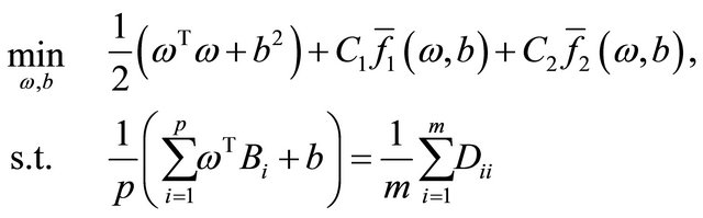 (1)
(1)
where
 and
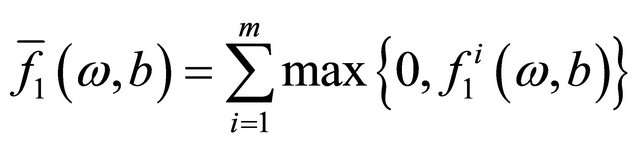
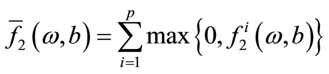
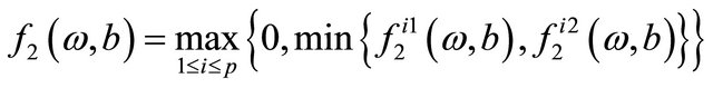
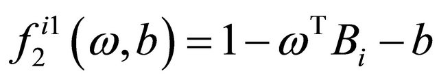
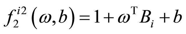
and  are loss functions corresponding to the labeled data and unlabeled data respectively and defined as follows,
where  denotes the absolute value of
 . The constraint is called balanced constraint that is used to avoid unbalanced solutions which classify all the unlabeled points in the same class.
For arbitrary vector , there lies an equivalent relation between its 1-norm and inf-norm in the sense that
 , then the sum term of model (1)
can be substituted by the inf-norm form and model (1) can be reformulated as follows,
 (2)
(2)
where
 .
.
We rewrite the constraint into the objective as a barrier term and reformulate  into its equivalent formulation
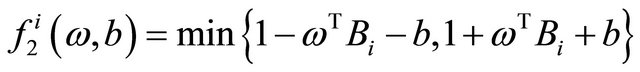 , and then obtain the following formulation that is our goal in the paper.
 (3)
(3)
where


 is a barrier parameter.
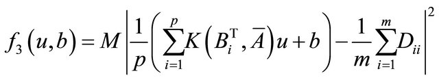
If the dataset is nonlinear separable, we need construct a surface separation based on some kernel trick (detailed discussion of it can be seen from [2] and etc.). Denote , assume that the surface we want to find is
 , where
  is usually taken as Gaussian kernel function with the form of
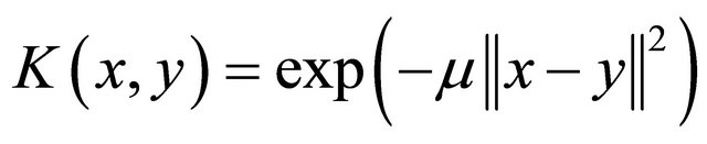
 is the kernel parameter,
 . To find the nonlinear decision surface, we need to solve the following problem:
 (4)
(4)
where


2.1. Aggregate Function and Aggregate Homotopy Method
Aggregate function is an attractive smooth approximate function. It has been used extensively for the the nonsmooth min-max problem [4], variational inequalities [6], mathematical programm with equilibrium constraints (MPEC) [16], non-smooth min-max-min problem [6] and etc. In the following, we will utilize the approximate function with its modification to establish an globally convergent method, called as aggregate homotopy method, for solving model (3) or (4).
In short, let  (or,
(or,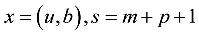 ) and denote model (3) or (4) as the following unified formulation:
 (5)
(5)
where
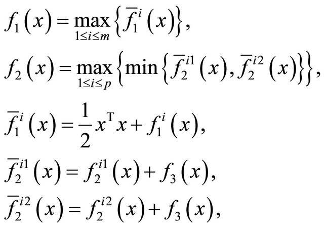 (6)
(6)
and  are defined as (3) or (4).
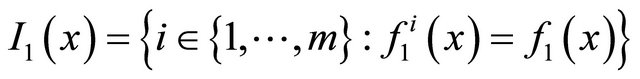
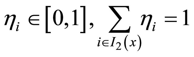
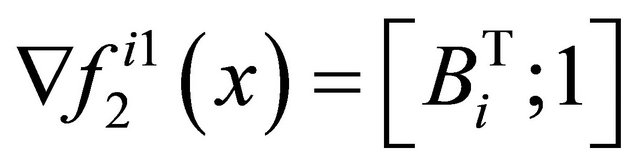
Denote , based on the optimality condition of non-smooth optimization theory in [9], we know that the subdifferential of
  and
and  can be computed as follows,
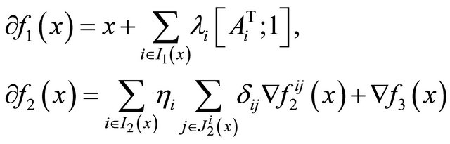 (7)
(7)
where


moreover, a point  can be called a stationary point or a solution point of (5) if satisfying
 .
.
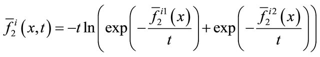
To solve model (5) by an aggregate homotopy method, we first introduce the following two smoothing functions,
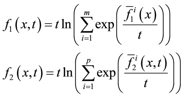 (8)
(8)
where  is defined as (6) and
 .
.
We call  and
and  as aggregate function and twice aggregate function respectively. The two smoothing functions have many good properties such as uniform approximation and etc. More details can be seen from [19].
Using above two uniformly approximations functions in (8), we define the following homotopy mapping:
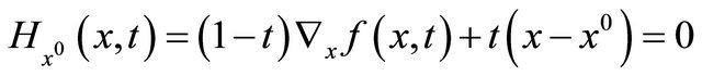 (9)
(9)
where  is an arbitrarily initial point and
 .
.
We call Equation (9) as an aggregate homotopy equation. It contains two limiting problems. On the one hand as , it has a unique solution
 . On the other hand, as
 , the solution of it approaches to a stationary point of (5), i.e., a solution
  satisfying
 .
.
For a given initial point , we denote the zeros point set of the aggregate homotopy mapping
  as
as
 (10)
(10)
It can be proved that  includes a smooth path
  with no bifurcation points, starting from
  and approaching to the hyperplane
  that leads to a solution of the original problem [21].
3. Inexact Predictor-Corrector Implementation of the Aggregate Homotopy Method
The path-following of the homotopy path  can be implemented by some predictor-corrector procedure. Some detailed discussion on the predictor-corrector algorithm with the convergence can be seen from [3,8] and etc. In the following, we first give the framework of the predictor-corrector procedure in this paper, and then discuss how to make an inexact predictor-corrector implementation.
3.1. Predictor-Corrector Path-Following Algorithm
Parameters. initial stepsize , maximum stepsize
 , minimum stepsize
 , stop criteria
  for procedure terminated, stop criteria
  for Newton corrector stopped, criteria
  for judging corrector plane, counter
 .
.
Data. Step 0.
 ,
,  ,
, .
.
Step 1. Compute a predictor point 
1) Solve the following linear equation
to obtain a unit tangent vector ;
;
2) ;
; ;
;
3) If  or
or ,
,  , return to 2); else, go to Step 2;
Step 2. Compute a corrector point 
1) If , take
  and
and ; else, take
 . Go to 2);
2) Solve equation
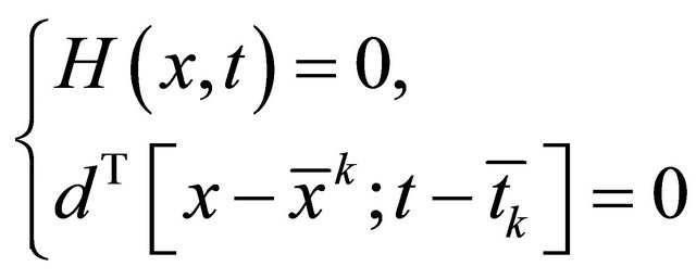
by Newton method with the stopping criteria  and go to 3);
3) If Newton corrector fail,  , go to 2); else, denote the solution as
 , go to 4);
4) If  or
or ,
,  , go to 2); else, go to 5);
5) If , stop ; else
 , k = k + 1, go to 6);
6) . If
. If  and the iteration number of Newton corrector is less than 3, go to 7); else , go to 1);
7) ,
, ; go to 1).
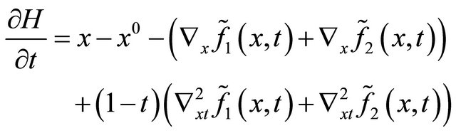
Notice that, the main computation cost of Algorithm 3.1 lies in the equations solver in Step 1) and 2), some inexact computation technique can be introduce to save the computation cost of them. we take the following approximate homotopy equation  with its Jacobian
  in place of the original
  with
with  during the computation of step 1) and 2).
Given parameters ,
,  , denote
 ,
,  ,
,

where
It’s proven in [20] that, only if the error  and
and  are small enough, or equivalently,
  and
and  are chosen appropriately, the approximate Euler-Newton predictor-corrector also approaches to a solution of original problem. Here we only list the main results and omit the proofs.
Denote
and ,
,  is the unit tangent vector obtained by the approximate computation,
  is the tangent vector by exact Euler predictor, we have the following lemma to guarantee the efficiency of the approximate tangent vector.
3.2. Lemma
For a given , if
, if  is small enough and satisfies

The approximate unit predictor tangent vector  is effective, i.e.,
  still makes a direction with arclength increased.
During the correction process, the following equation must be solved
 (11)
(11)
where  is an appropriate predictor point obtained from the former predictor step. We adopt the following approximate Newton method to solve (11),
 (12)
(12)
where

From 0 is a regular value of  and
and  is a unit tangent vector induced by
 , we know, if the step
  is chosen appropriately, the equation (11) has a solution and the approximate Newton iteration (12) is effective.
3.3. Approximate Newton Corrector Convergence Theorem
Suppose that  have solution
  with nonsingular
 , there exists a neighborhood
  and
and , for any
 , if for each
 ,
,  and
and  satisfying
 .
.
Then the approximate Newton iteration point sequence  from (12) is well defined and converges to
 .
.
4. Numerical Results
In this section, some numerical examples and comparisons are given to illustrate the efficiency of our method. Two artificial datasets are generated first. The first one consists of 34 points generated by “rand” function, 14 of them are labeled and the remaining 30 are seen as unlabeled data. The second one consists of 242 points taken from two nonlinear bihelix curves that are generated by , where one is obtained by taking
 , the other is by taking
 ,
, . We take randomly
  of them as labeled and the remaining
  as unlabeled. The comparisons of our method with the LSVM method from [15] without the consideration of unlabeled data are given. Final results are illustrated in Figures 1 and 2.

Figure 1. Result on linear artificial data of LSVM and the new algorithm.

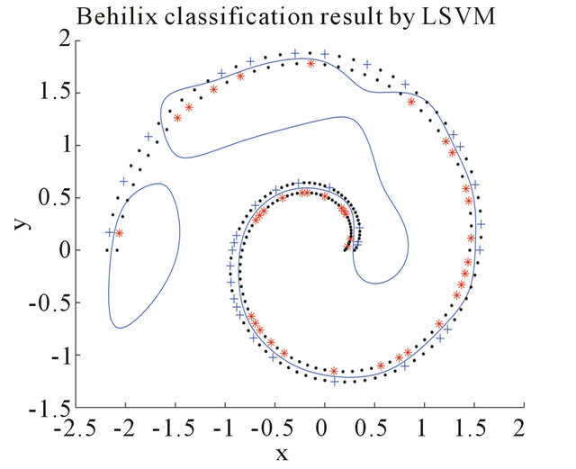
Figure 2. Result on nonlinear bihelix curve artificial data of LSVM and the new algorithm.
To reveal the efficiency of our algorithm for S3VMs, comparisons of our algorithm (InSH) with some other existing algorithms for S3VMs such as the convexconcave procedure in [5] (vS3VM), the continuation method in [12] (cS3VM) and the gradient descent method in [13] ( S3VM), are given for some standard test data from [10]. For the linear programming subproblem arising in [5], we solve it with the Matlab function
  in optimization toolbox. The comparison results are listed in the following Table 1.
Table 1. Comparison Results on test data (test error %).
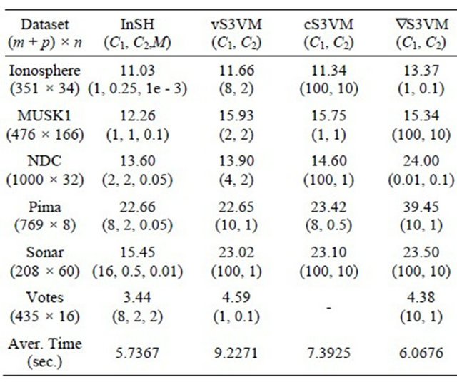
-: denotes the method fails for the dataset.
All the computations are performed on a computer running the software Matlab 7.0 on Microsoft Windows Vista with Intel(R) Core(TM)2 Duo CPU 1.83 GHz processor and 1789 megabytes of memory. During the computation, we take ,
,  ,
,  ,
,  ,
,  ,
,  ,
,  ,
,  are taken as the one for the least test error. If necessary, the kernel parameter
  is taken the best leads to the least test error among
 . The parameters for determining the inexact index set are taken as
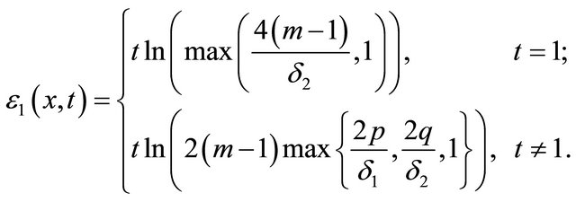
where ,
,  ,
,  and
and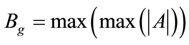 .
.  has the same expression as
  where
where  and
and .
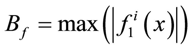
.  and
and  are taken as
  that are given to bound the error of
  and
and .
.
5. Acknowledgements
The research was supported by the National Nature Science Foundation of China (No. 11001092) and the TianYuan Special Funds of the National Natural Science Foundation of China (Grant No. 11226304).
REFERENCES
- A. Astorino and A. Fuduli, “Nonsmooth Optimization Techniques for Semi-Supervised Classification,” IEEE Transactions on Pattern Analysis and Machine Intelligence, Vol. 29, No. 12, 2007, pp. 2135-2142. doi:10.1109/TPAMI.2007.1102
- C. J. C. Burges, “A Tutorial on Support Vector Machines for Pattern Recognition, “Data Mining and Knowledge Discovery, Vol. 2, No. 2, 1998, pp. 121-167. doi:10.1023/A:1009715923555
- E. L. Allgower and K. Georg, “Numerical Continuation Methods: An Introduction,” Springer-Vergal, Berlin, 1990. doi:10.1007/978-3-642-61257-2
- E. Polak, J. O. Royset and R. S. Womersley, “Algorithms with Adaptive Smoothing for Finite Minimax Problems,” Journal of Optimization Theory and Application, Vol. 119, No. 3, 2003, pp. 459-484. doi:10.1023/B:JOTA.0000006685.60019.3e
- G. Fung and O. Mangasarian, “Semi-Supervised Support Vector Machines for Unlabeled Data Classification,” Optimization Methods and Software, Vol. 15, No. 1, 2001, pp. 29-44. doi:10.1080/10556780108805809
- G. X., Liu, “Aggregate Homotopy Methods for Solving Sequential Max-Min Problems, Complementarity Problems and Variational Inequalities,” PhD Thesis, Jilin University, Jilin, 2003.
- K. Bennett and A. Demiriz, “Semi-Supervised Support Vector Machines,” In: M. S. Kearns, S. A. Solla and D. A. Cohn, Eds, Advances in Neural Information Processing Systems, MIT Press, Vol. 10, 1998, pp. 368-374.
- L. T. Watson, S. C. Billups and A. P. Morgan, “Algorithm 652 Hompack: A Suite of Codes for Globally Convergent Homotopy Algorithms,” ACM Transactions on Mathematical Software, Vol. 13, No. 3, 1987, pp. 281- 310. doi:10.1145/29380.214343
- M. M. Mkela and P. Neittaanmki, “Nonsmooth Optimizatin: Analysis and Algorithms with Application to Optimal Control,” Utopia Press, Singapore, 1992.
- P. M. Murphy and D. W. Aha, “UCI Repository of Machine Learning Databases. http://www.ics.uci.edu/ mlearn/MLRepository.html.
- O. Chapelle, V. Sindhwani and S. S. Keerthi, “Optimization Techniques for Semi-Supervised Support Vector Machines,” Journal of Machine Learning Research, Vol. 9, 2008, pp. 203-233.
- O. Chapelle, M. Chi and A. Zien, “A Continuation Method for Semi-Supervised SVMs,” ACM International Conference Proceeding Series, Proceedings of the 23rd international conference on Machine learning, Vol. 148, 2006, pp. 185-192.
- O. Chapelle and A. Zien, “Semi-Supervised Classification by Low Density Separation,” Proceedings of the Tenth International Workshop on Artificial Intelligence and Statistics, Vol. 1, 2005, pp. 57-64.
- O. Chapelle, V. Sindwani and S. Keerthi, “Branch and Bound for Semi-Supervised Support Vector Machines,” Advances in Neural Information Processing Systems 19, Proceedings of the 2006 Conference, MIT Press, Cambridge, 2007, pp. 217-224.
- O. L. Mangasarian and D. R. Musicant, “Lagrangian Support Vector Machines,” Journal of Machine Learning Research, Vol. 1, 2001, pp. 161-177.
- S. Birbil, S. C. Fang and J. Han, “Entropic Regularization Approach for Mathematical Programs with Equilibrium Constraints,” Technical Report, Industrial Engineering and Operations Research, Carolina, 2002.
- T. D. Bie, N. Cristianini, “Semi-Supervised Learning Using Semi-Definite Programming,” In: O. Chapelle, B. Scholkopf and A. Zien, Eds., Semi-Supervised Learning, MIT Press, Cambridge, 2006.
- X. J. Zhu, “Semi-Supervised Learning Literature Survey,” Technical Report 1530, Computer Science, University of Wisconsin-Madison, 2005.
- X. S. Li and S. C. Fang, “On the Entropic Regularization Method for Solving Min-Max Problems with Applications,” Mathematical Methods and Operations Research, Vol. 46, No. 1, 1997, pp. 119-130. doi:10.1007/BF01199466
- Y. Xiao, H. J. Xiong and B. Yu, “Truncated Aggregate Homotopy Method for Nonconvex Nonlinear Programming,” Optimization Methods and Software, 2012, pp. 1- 18.
- H. J. Xiong and B. Yu, “Aggregate Homotopy Method for Semi-Supervised SVMs,” 2011 International Conference on Electric Information and Control Engineering, pp. 1147-1150.