Open Journal of Modelling and Simulation
Vol.2 No.4(2014), Article
ID:49623,14
pages
DOI:10.4236/ojmsi.2014.24013
Mathematical Modelling of Population Growth: The Case of Logistic and Von Bertalanffy Models
Mohammed Yiha Dawed, Purnachandra Rao Koya, Ayele Taye Goshu*
School of Mathematical and Statistical Sciences, Hawassa University, Hawassa, Ethiopia
Email: mhmmdyiha@yahoo.com, drkpraocecc@yahoo.co.in, *Ayele_taye@yahoo.com
Copyright © 2014 by authors and Scientific Research Publishing Inc.
This work is licensed under the Creative Commons Attribution International License (CC BY).
http://creativecommons.org/licenses/by/4.0/


Received 16 July 2014; revised 20 August 2014; accepted 6 September 2014
ABSTRACT
In this paper, some theoretical mathematical aspects of the known predator-prey problem are considered by relaxing the assumptions that interaction of a predation leads to little or no effect on growth of the prey population and the prey growth rate parameter is a positive valued function of time. The predator growth model is derived considering that the prey follows a known growth models viz., Logistic and Von Bertalanffy. The result shows that the predator’s population growth models look to be new functions. For either models, the predator population size either converges to a finite positive limit or to 0 or diverges to +∞. It is shown algebraically and illustrated pictorially that there is a condition at which the predator-prey population models both converge to the same finite limit. Derivations and simulation studies are provided in the paper. Analysis of equilibrium points and stability is also included.
Keywords:Predator-Prey, Koya-Goshu, Logistic, Population Growth, Von Bertalanffy

1. Introduction
Growth models have been widely studied and applied in many areas especially animal, plant and forestry sciences [1] -[7] . A generalized mathematical model for biological growth is introduced in [7] which includes the known functions such as Generalized Logistic, Particular Case of Logistic, Richards, Von Bertalanffy, Brody, Logistic, Gompertz, Generalized Weibull, Weibull, Monomolecular, Mitscherlich and many more new models. These are derived as solutions of the rate-state first order ordinary differential equation. Detailed studies of these models with their respective relative growth models are given in [7] -[9] .
The growth models are so flexible to be useful in modelling problems. In this paper, we apply some of these growth models to the population dynamics, especially the predator-prey problems. We consider that the growth of prey population size or density follows biological growth models and construct the corresponding growth models for the predator.
In the next sections, the Lotka-Volterra predator-prey model is presented in Section 2 and the newly proposed approach in Section 3. The case of logistic prey model is considered in Section 3.1 and that of Von Bertalanffy in Section 3.2. Conclusions are in Section 4.
2. Lotka-Volterra Predator-Prey Models
The classical model of a predator-prey problem was originally developed in the 1920s by Vito Volterra, and since then many related studies have been conducted [10] -[14] .
The Lotka-Volterra predator-prey equations are first-order and nonlinear differential equations defined [10] as:
 . (1)
. (1)
In the classical model,  are all positive constants. Assumptions of the model are the following:
1) In absence of predator, prey population would grow at a natural rate.
2) In absence of prey, predator population would decline or grow at a natural rate.
3) When both the predator and prey are present, there occur, in combination with these natural rates of growth and decline, a decline in the prey population and a growth in the predator population each at a rate proportional to the frequency of encounters between individuals of the two populations. We often assume further that the frequency of such encounters is proportional to the product of the populations.
Other assumptions [13] consider about environment and evolution of the predator and prey populations as follows:
1) The prey population finds ample food at all times.
2) The food supply of the predator population depends entirely on the size of the prey population.
3) The rate of change of population is proportional to its size.
4) During the process, the environment does not change in favor of one species and the genetic adaptation is sufficiently slow.
5) Predators have limitless appetite.
The usual assumption of constants for the parameters a, b, c, d may lead to oversimplification of the system and yet not be realistic [10] [11] [14] . In particular, [14] recommends that these parameters can be functions of time.
Moreover, there are some studies that indicate that predation may promote, hinder or have no effect on interspecific competitive interactions and the probability of prey coexistence [11] [15] [16] . This can be affected by the mechanisms of predation and competition together with what we measure from the process. According the authors, predators may lead to an increase of the strength of interspecific competitions or its impact on a prey population; or happen to decrease competitive strength or impact; or in other cases, have very little effect on the competitive interactions.
This means the ecosystem is so complex that the prey and predator interactions can lead to various outcomes. This paper considers the case when this interaction leads to a little or no effect on growth of the prey population.
3. The Proposed Model
Here we consider the case when the interaction of the prey and predator populations leads to a little or no effect on growth of the prey population, that is, . Moreover, we assume the parameter
 ![]() is positive valued function of time. By these considerations, the assumptions of the classical predator-prey model are relaxed. Then the newly proposed predator-prey model is defined as follows:
is positive valued function of time. By these considerations, the assumptions of the classical predator-prey model are relaxed. Then the newly proposed predator-prey model is defined as follows:
 (2)
(2)
where ![]() is population size or density of prey;
is population size or density of prey; ![]() is population size or density of predator communities in the system. Here we assume
is population size or density of predator communities in the system. Here we assume  to be a relative growth rate function which is positive valued function of time
 . The other parameters
  are considered to be positive constants.
The prey equation in (2) is the first order differential equations whose solutions are studied to be growth models in [8] . This leads that the prey model can be selected from the large family of growth functions and solve for the predator equation. This will give more options for researchers and practitioners who are working in field of population dynamics.
The general approach is as follows:
1) Assume that there is prior information about the prey population that ![]() is a known growth function.
is a known growth function.
2) Assume that the impact of predator on prey population growth is negligible.
3) Predator population declines in absence of prey.
4) The predator population grows with a rate proportional to a function of both ![]() and
and![]() , i.e.,
, i.e.,  .
.
5) Solve for predator’s population size![]() .
.
The idea is to consider the prey population to follow a known growth model among the family of KoyaGoshu models, and then construct the corresponding growth model for the predator population. This is can be helpful, for example, for managing the ecosystem. Here we consider Logistic and Von Bertalanffy growth models for prey population and solve for the respective predator population sizes.
3.1. Logistic Prey Model
We assume that the growth of prey population follows Logistic growth function and construct the corresponding predator growth model. Thus, the prey population growth is assumed to be described by Logistic model given as follows:
 (3)
(3)
where ,
,  is initial prey population,
  is asymptotic growth of prey population, and
 is absolute growth rate. The Logistic curve has a single point of inflection at time
  and when the growth reaches half of its asymptotic growth
 . The respective relative growth rate is
 . Detailed discussion is found in [7] -[9] .
After substituting (3) in (2), the corresponding predator’s population growth function is derived to be:
 (4)
(4)
here  is the initial predator population size. Derivation is given in Appendix 1. It is interesting to find that prey and predator models are related as in (4) or as in (5):
 . (5)
. (5)
The predator model  in equation (4) looks a new function and it does not match any one of the commonly known growth models.
It is found that this predator model either declines and converges to a finite positive limit or converges to 0 or diverges to ![]() depending on the values of the birth parameter
depending on the values of the birth parameter ![]() and death parameter
and death parameter ![]() of the predator. These three cases are discussed here below.
of the predator. These three cases are discussed here below.
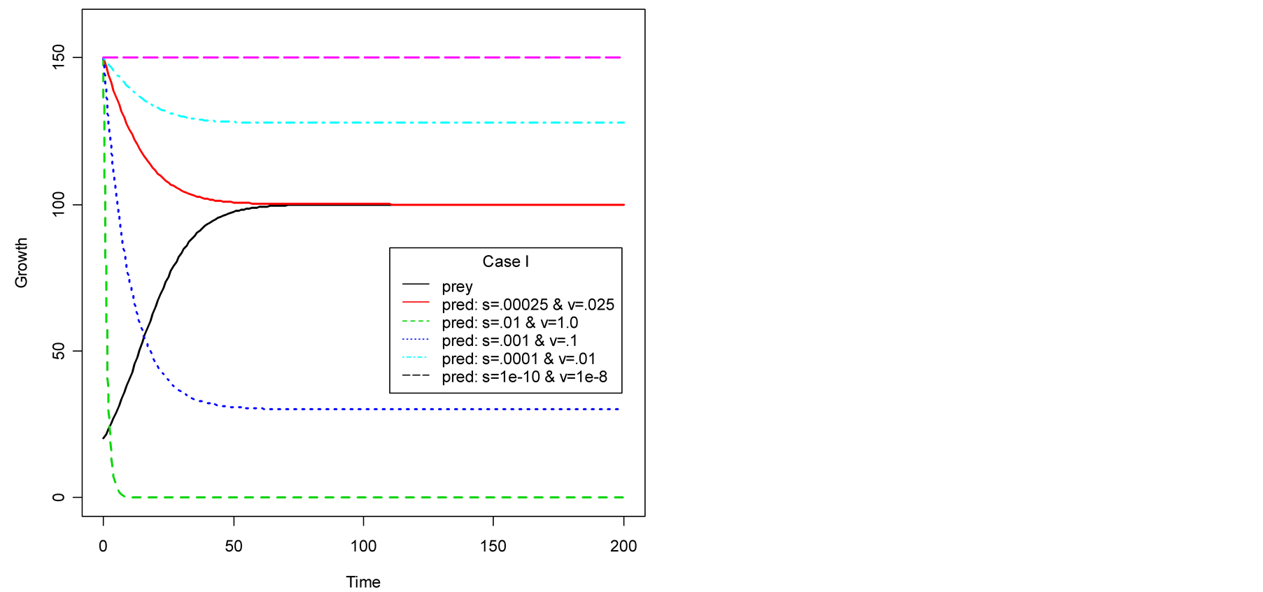
Case I (As = v): In this case,  or equivalently
  and also
 . It can be interpreted that the predator population decays to lower asymptote or grows to upper asymptote given by
 , while the prey grows following Logistic curve and reaches the upper asymptote
  (see Figure 1(a)).
It is interesting to find that the two populations converge to same size when birth rate of predator becomes:
 (6)
(6)
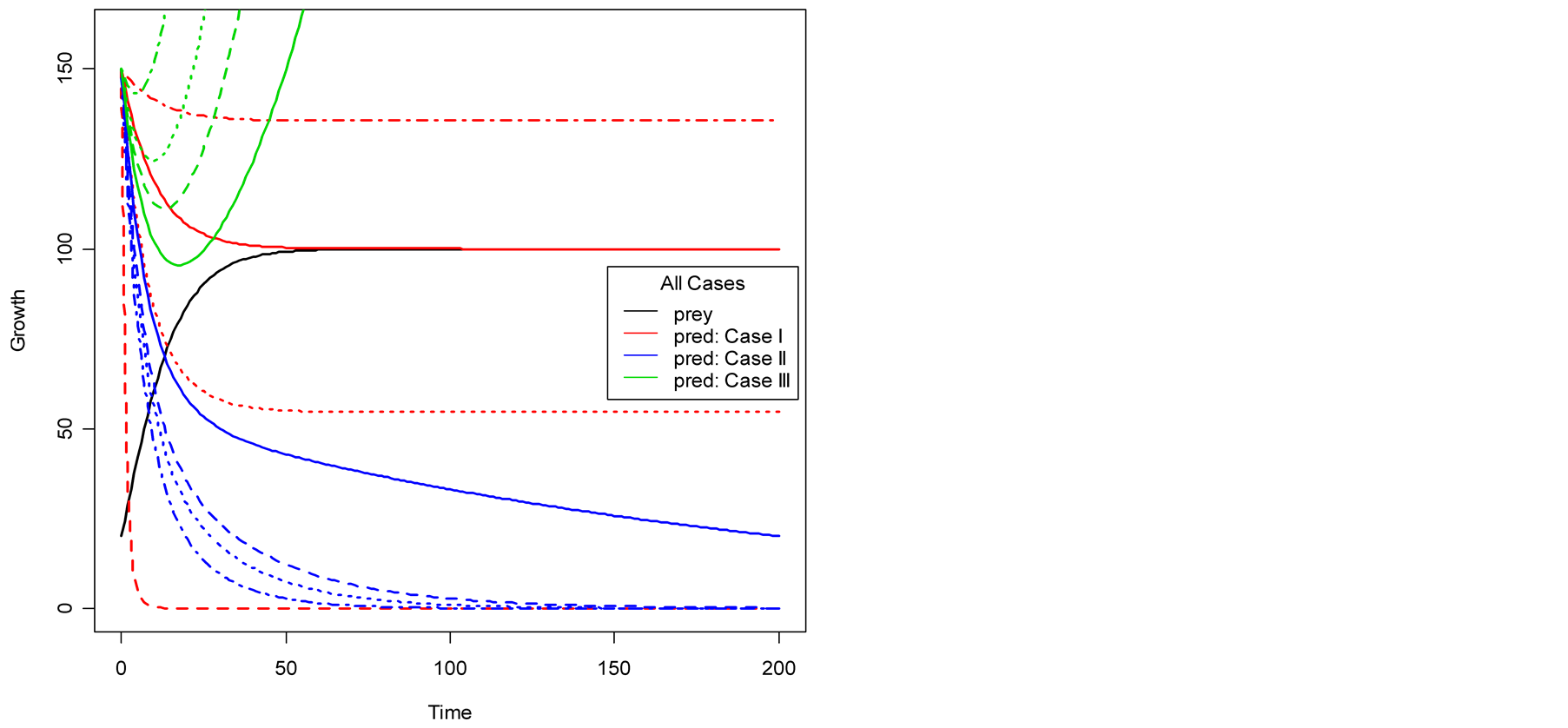
then the prey population’s upper asymptote and the predator population’s lower asymptote coincide at  and continue to maintain the same and equivalent population size. Figure 1(a) illustrates this occasion. When initial size of the predator is smaller than A, then there is an increment of its growth to converge to the same size of prey. Plots are shown in Figure 2.
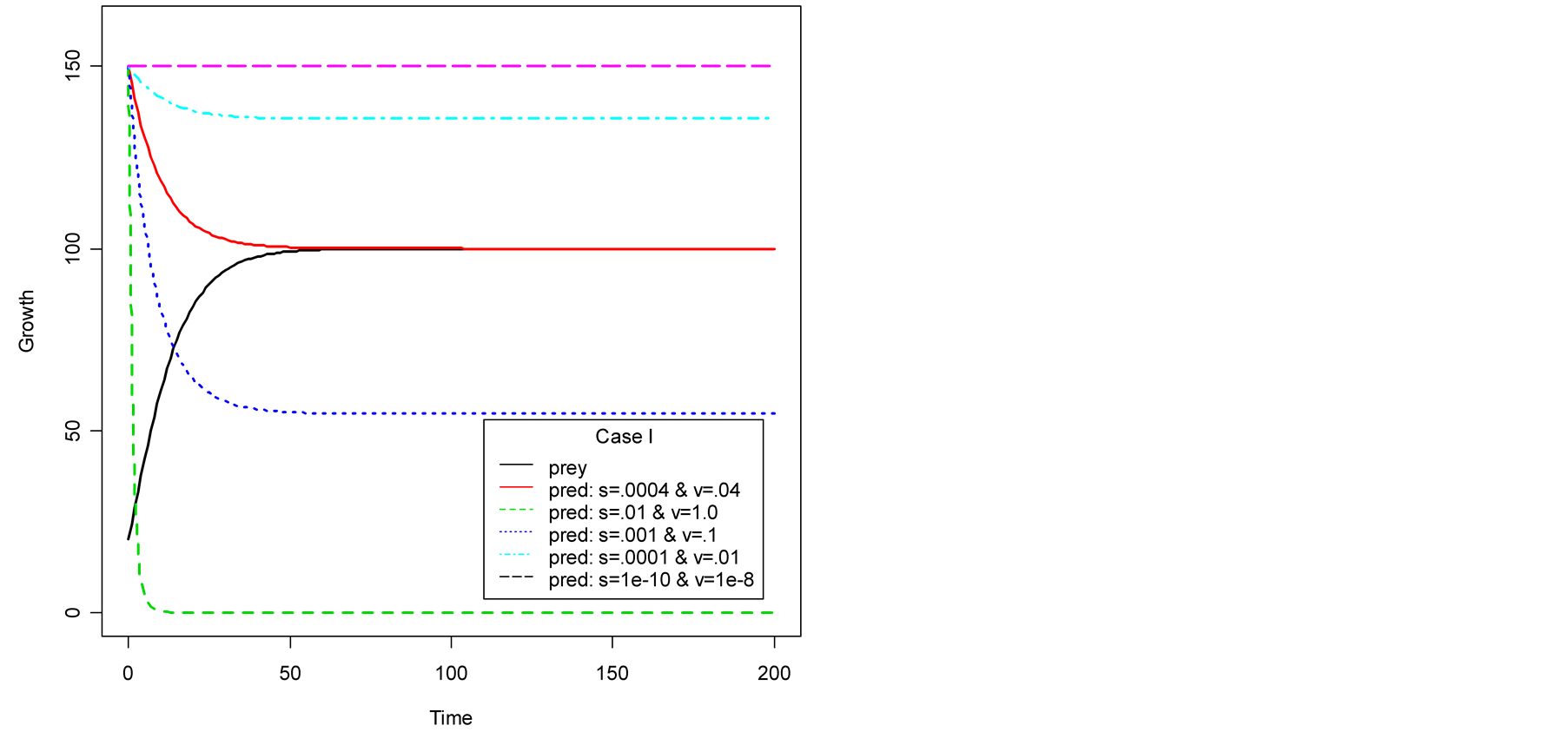
Case II (As < v): In this case, the predator population decays and eventually declines down to 0, while the prey population remains to follows logistic growth model and approaches an upper asymptote  (see Figure 1(b)).
Case III (As > v): In this case, the predator population declines for a while and grows higher and eventually diverges![]() , while the prey population follows logistic model and grows to an upper asymptote
, while the prey population follows logistic model and grows to an upper asymptote  (see Figure 1(c)).
3.2. Simulation Study
The simulation study is designed in by varying the model parameters:  for prey and
  for predator population; and the two models viz. Logistic and Von Bertalanffy each with three cases.
Model: Logistic, Von Bertalanffy.
Prey’s parameters: ,
,  ,
, .
.
Predator’s parameters: .
.
Cases: Case I: , Case II:
 , Case III:
 .
.
Case I:  &
& ;
;  &
& ;
;  &
& ;
;  &
&  .
.
Case II:  &
& ;
;  &
& ;
;  &
& ;
;  &
&  .
.
Case III:  &
& ;
; &
& ;
;  &
& ;
;  &
& .
.
The specifications are as follows:
Figure 1(a) displays Case I, where death/birth of predator is equal to A. The birth rate is varied from smaller to larger values. It is seen that the predator population size declines and eventually converges to a positive quantity with various speeds of declines. More results are plotted in Figure 2. Figure 1(b) displays Case II, where death/birth of predator is greater than A. The death rate is increased from smaller to larger values. The predator population declines with speed and eventually converges to zero. More results are plotted in Figure 2.
In Case III, see Figure 1(c), the death/birth of predator is less than A. As shown by simulations plotted in Figure 1 and Figure 2, the predator population declines for some time and then increases to infinity. The minimal point at which the curve turns or gets minimum value is found to be: . Then the values of
 (a)
(a) (b)
(b) (c)
(c)
Figure 1. Plots of predator population dynamics with prey population growth following logistic model (a) Case I, (b) Case II and (c) Case III.
prey and predator populations are  and
and , respectively.
In summary, it is observed that the predator population either converges to a finite limit or converges to 0 or diverges to ![]() depending on the selection of the parameters. We show by simulation study that for a particular value of the birth parameter
depending on the selection of the parameters. We show by simulation study that for a particular value of the birth parameter![]() , the population sizes of both the prey and predator will converge to the same asymptote.
, the population sizes of both the prey and predator will converge to the same asymptote.
4. Analysis of Phase Diagram and Equilibrium Points
The newly proposed predator-prey model (2) in its full form can be expressed, in case of Logistic prey, as the system of equations  and
and . The two equilibrium points of this system are
 (a)
(a) (b)
(b)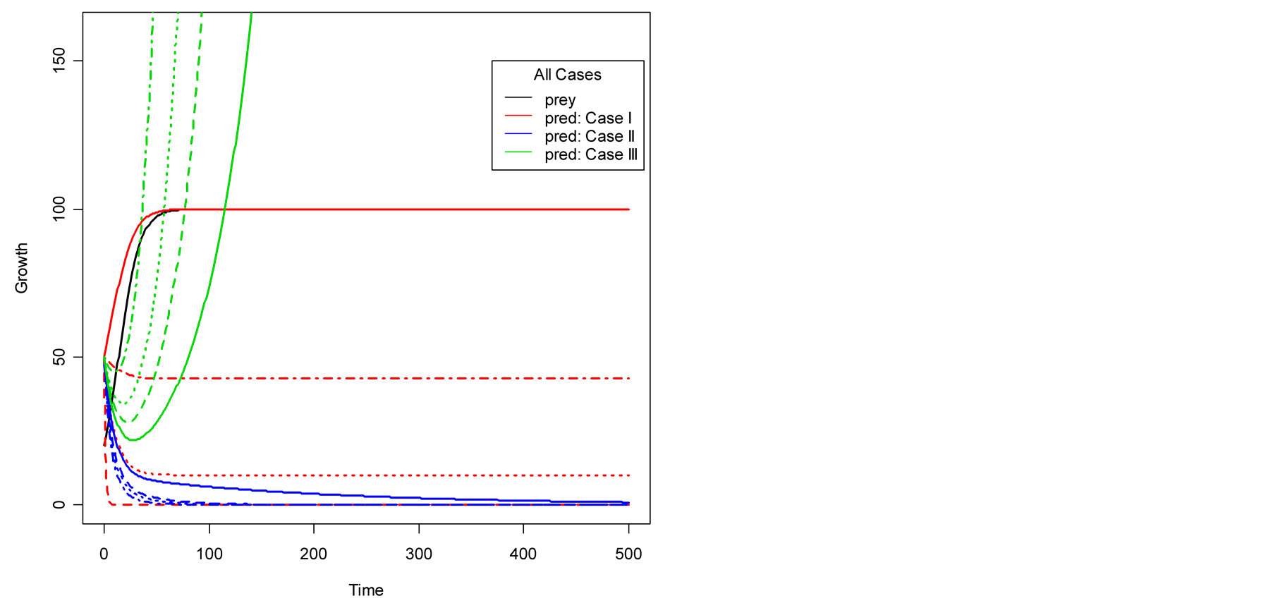 (c)
(c)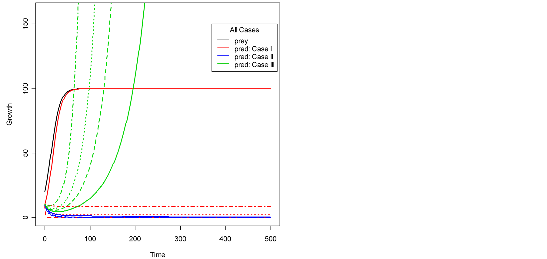 (d)
(d)
Figure 2. Plots of all three cases for the predator population dynamics with prey population growth following logistic model (a)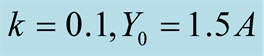 ; (b)
; (b) ; (c)
; (c) ; (d)
; (d) .
.
found to be  and
and  since at both these points the necessary and sufficient conditions
  and
and  are satisfied. Also the Jacobian matrix of the system of equations is
 . We now analyze the nature of the equilibrium points as in [12] and the summery is tabulated in Table1
Nature of the equilibrium point : The Jacobean matrix at this point takes the form
 . The eigenvalues are
  and
and . Recall that both the parameters

Table 1. Stability of the equilibrium points—the case of logistic prey model.
and ![]() are positive quantities. Thus, the eigenvalues are real and opposite in sign and hence the equilibrium point
are positive quantities. Thus, the eigenvalues are real and opposite in sign and hence the equilibrium point  is unstable.
Nature of the equilibrium point : The Jacobean matrix becomes
 . The eigenvalues are
  and
and . Recall that the parameters
  and
and  are positive quantities and thus here arise three cases. Case I
 : In this case
 is negative and
  is zero and hence the equilibrium point
  is stable.
Case II : In this case both the eigenvalues
  and
and  are negative and hence the equilibrium point
  is stable. Case III
 : In this case both the eigenvalue
  is negative while
  is positive and hence the equilibrium point
  is unstable.
4.1. Von Bertalanffy Prey Model
In this section, we assume that the growth of prey follow Von Bertalanffy biological growth function and construct the corresponding predator growth model.
Thus, the prey population growth is assumed to be described by Von Bertalanffy as
 (7)
(7)
where ,
,  is initial prey population,
  is asymptotic growth of the prey populationand
  is absolute growth rate parameter. A single point of inflection occurs when the growth reaches the weight
  at time
 . Its relative growth rate function is
 . Further analyses are available in [7] -[9] .
Now then, by substituting (7) in (2), we determine the corresponding predator population growth function (see Appendix 2) as:
 (8)
(8)
here  is the initial predator population size. It is interesting to observe that both population growth functions of prey and predator are related as (8) or as (9):
 (9)
(9)
The three cases are presented below.
Case I (As = v): In this case  and
and
 . It can be interpreted that the predator population decays with an exponential rate of
  and converges to a lower asymptote of
 . The prey population grows following Von Bertalanffy model and reaches the upper asymptote
  (see Figure 3(a)). The situation at which the prey population upper asymptote and the predator population lower asymptote coincide at
  and continue to maintain the same population sizes is found to be:
 . (10)
Figure 3(a) also illustrates the occasion where the two populations converge to same. When initial size of the predator is smaller than A, then there is an increment of its growth to converge to the same size of prey. See Figure 4(c), Figure 4(d).
Case II (As < v): In this case, the predator population decays and eventually dies down to 0, while the prey population follows Von Bertalanffy, as assumed, and reach an upper asymptote  (see Figure 3(b)).
Case III (As > v): In this case, the predator population grows higher and higher and eventually diverges to![]() , while the prey population grows according to the Von Bertalanffy curve with an upper asymptote of
, while the prey population grows according to the Von Bertalanffy curve with an upper asymptote of  (see Figure 3(c)). The predator population growth has minimum value at time point
  that is a function of the parameters. It is given by:
 . Then the values of prey and predator populations are, respectively,
  and
and
 .
.
4.2. Simulation Study
Similar simulation study is conducted for the Von Bertalanffy model case, using the design suggested in subsection 3.1. The results are displayed in Figure 3 and Figure 4. Figure 3(a) displays Case I for Von Bertalanffy
 (a)
(a)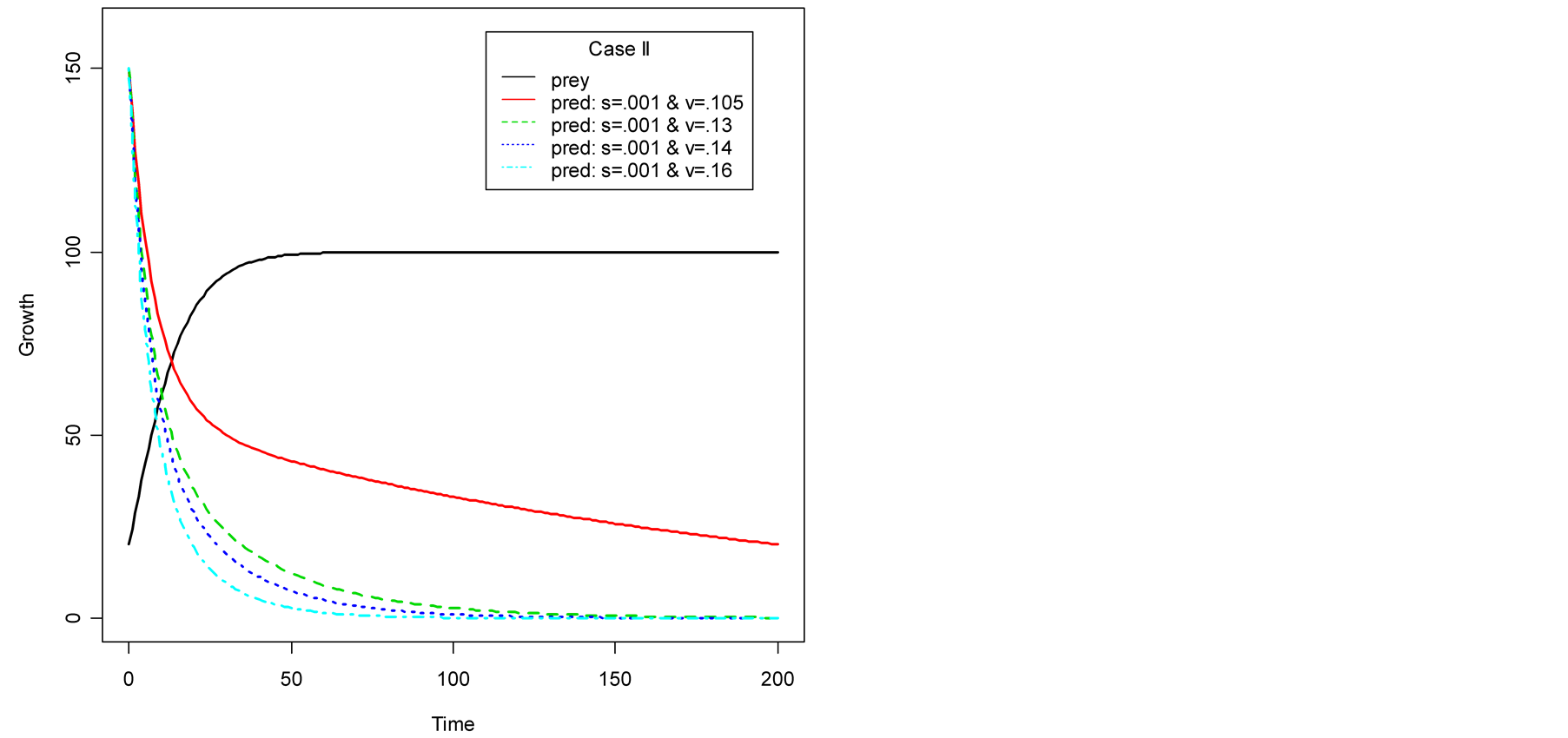 (b)
(b) (c)
(c)
Figure 3. Plots of predator population dynamics with prey population growth following Von Bertalanffy model (a) Case I, (b) Case II and (c) Case III.
case, where death/birth of predator is equal to A. The birth rate is varied from smaller to larger values. It is seen that the predator population size declines and eventually converges to a positive quantity with various speeds of declines. Other simulated results are plotted in Figure 4.
Figure 3(b) displays Case II, where death/ birth of predator is greater than A. The death rate is increased from smaller to larger values. The predator population declines with speed and eventually converges to zero. In Case III, see Figure 3(c), the death/birth of predator is less than A. The predator population declines for some time and then increases to infinity. In summary, the predator model either declines and converges to a finite positive limit or converges to 0 or diverges to ![]() depending on the values of the birth parameter s and death parameter v of the predator. More results are given in Figure 4.
depending on the values of the birth parameter s and death parameter v of the predator. More results are given in Figure 4.
5. Analysis of Phase Diagram and Equilibrium Points
The newly proposed predator-prey model (2) in its full form can be expressed, in case of Von Bertalanffy prey,
 (a)
(a)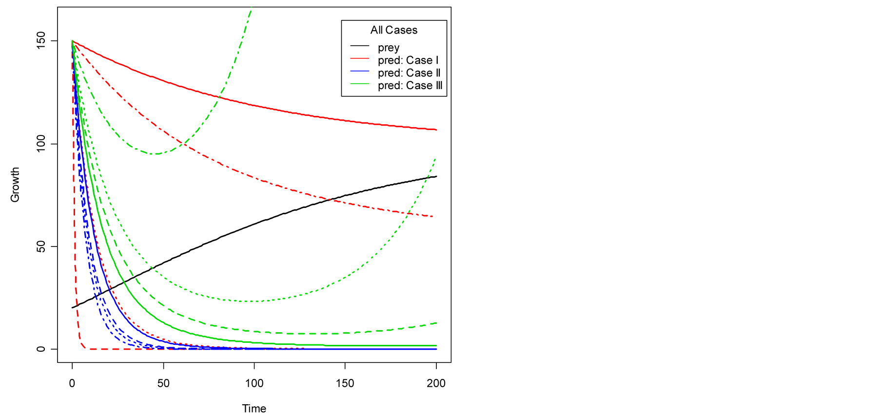 (b)
(b)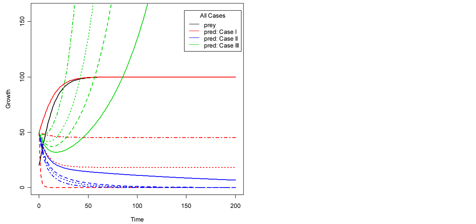 (c)
(c) (d)
(d)
Figure 4. Plots of all three cases for the predator population dynamics with prey population growth following Von Bertalanffy model (a) ; (b)
; (b) ; (c)
; (c) ; (d)
; (d) .
.
as the system of equations  and
and . The two equilibrium points of this system are found to be
  and
and  since at both these points the necessary and sufficient conditions
  and
and  are satisfied. Also the Jacobian matrix of the system of equations is
 . We now analyze the nature of the equilibrium points below as in [12]
and the summery is tabulated in Table2
Nature of the equilibrium point : The Jacobean matrix at this point takes the form
 and the corresponding eigenvalues are
 and
and . Recall that all the parameters
  and
and ![]() are positive quantities and thus here arise the following three cases: Case I
are positive quantities and thus here arise the following three cases: Case I  or
or . In this case
is zero while  is negative and hence the equilibrium point
  is stable. Case II
 or
or . In this case both the eigenvalues
  and
and  are negative and hence the equilibrium point
  is stable. Case III
  or
or
 . In this case the eigenvalue
  is positive while
  is negative and hence the equilibrium point
  is unstable.
Nature of the equilibrium point : The Jacobean matrix at this point takes the form
 and the corresponding eigenvalues are
  and
and .
.
Recall that the parameters  and
and  are positive quantities and thus here arise three cases: Case I
 : In this case
  is negative and
  is zero and hence the equilibrium point
 is stable. Case II
 : In this case both the eigenvalues
  and
and 
are negative and hence the equilibrium point  is stable. Case III
 : In this case both the eigenvalue
  is negative while
  is positive and hence the equilibrium point
 is unstable.
Table 2. Stability of the equilibrium points—the case of Von Bertalanffy prey model.
6. Conclusions
Some theoretical mathematical aspects of the well known predator-prey problem are studied. The classical assumptions are relaxed in that the interaction of a predation leads to little or no effect on growth of the prey population and the prey’s growth rate parameter is a positive valued function of time. The idea is implemented for the two cases that the prey population follows Logistic and Von Bertalanffy growth models. The respective predator models are derived and analyzed.
The simulation studies and further analysis of the models reveal that the predator population grows in such a way that either converges to a finite limit or 0 or diverges to +∞ irrespective of the fact that the prey population continuously grows and eventually converges to upper asymptote. There is a situation at which both prey and predator populations converge to the same amount, irrespective of their initial population sizes. There is also a situation where the predator population declines for some time and then starts to increase and diverges to infinity. Moreover, two equilibrium points are identified in each case, which are stable only under some specific conditions.
In general, the analytic and simulation studies have revealed some insights to the problem addressed in this paper so that the models obtained can be applied to the real-world situations.
References
- Von Bertalanffy, L. (1957) Quantitative Laws in Metabolism and Growth. Quarterly Review of Biology, 3, 218.
- Brody, S. (1945) Bioenergetics and Growth. Rheinhold Pub. Corp., NY.
- Eberhardt, L.L. and Breiwick, J.M. (2012) Models for Population Growth Curves. ISRN Ecology, 2012, Article ID: 815016. http://dx.doi.org/10.5402/2012/815016
- France, J., Dijkstra, J. and Dhanoa, M.S. (1996) Growth Functions and Their Application in Animal Science. Annales De Zootechnie, 45, 165-174. http://dx.doi.org/10.1051/animres:19960637
- Richards, F.J. (1959) A Flexible Growth Function for Empirical Use. Journal of Experimental Botany, 10, 290-300. http://dx.doi.org/10.1093/jxb/10.2.290
- Zeide, B. (1993) Analysis of Growth Equations. Forest Science, 39, 594-616.
- Koya, P.R. and Goshu, A.T. (2013) Generalized Mathematical Model for Biological Growths. Open Journal of Modelling and Simulation, 1, 42-53. http://dx.doi.org/10.4236/ojmsi.2013.14008
- Koya, P.R. and Goshu, A.T. (2013) Solutions of Rate-State Equation Describing Biological Growths. American Journal of Mathematics and Statistics, 3, 305-311.
- Goshu, A.T. and Koya, P.R. (2013) Derivation of Inflection Points of Nonlinear Regression Curves—Implications to Statistics. American Journal of Theoretical and Applied Statistics, 2, 268-272. http://dx.doi.org/10.11648/j.ajtas.20130206.25
- Barnes, B. and Fulford, G.R. (2009) Mathematical Modelling with Case Studies: A Differential Equations Approach Using Maple and Matlab. 2nd Edition.
- Chase, J.M., Abrams, P.A., Grover, J.P., Diehl, S., Chesson, P., Holt, R.D., Richards, S.A., Nisbet, R.M. and Case, T.J. (2002) The Interaction between Predation and Competition: A Review and Synthesis. Ecology Letters, 5, 302-315. http://dx.doi.org/10.1046/j.1461-0248.2002.00315.x
- Logan, J.D. (1987) Applied Mathematics—A Contemporary Approach. John Wiley and Sons, New York.
- http://en.wikipedia.org/wiki/Lotka%E2%80%93Volterra_equation
- Renshaw, E. (1991) Modeling Biological Populations in Space and Time. Cambridge University Press, Cambridge. http://dx.doi.org/10.1017/CBO9780511624094
- Yodzis, P. (1986) Competition, Mortality and Community Structure. In: Diamond, J.M. and Case, T.J., Eds., Community Ecology, Harper and Row, New York, 480-491.
- Gurevitch, J.J., Morrison, A. and Hedges, L.V. (2000) The Interaction between Competition and Predation: A Meta-Analysis of Field Experiments. The American Naturalist, 155, 435-453. http://dx.doi.org/10.1086/303337
Appendix 1: Derivation of Predator Model Given That Prey Follows Logistic Growth Model
Consider the predator equation


 .
.
We now substitute the Logistic function for the prey growth. That is
 ,
, .
.
Thus,
 .
.
Put, 

 .
.
Now, on substituting ![]() and
and , the
, the  takes the following transformation equation:
 .
.
Here  is an integral constant and that we determine as follows:
 .
.
Put . Then
 .
.


is the solution for the predator equation, representing predator’s population growth at t.
Appendix 2: Derivation of Predator Model Given That Prey Follows Von Bertalanffy Growth Model
Consider the predator equation
 .
.
We now substitute the Von Bertalanffy function for the prey growth. That is
 ,
, .
.
Thus,
 .
.
Put,

 .
.
Here  is an integral constant and that we determine as follows:
 .
.
Put . Then,

is the solution for the predator equation, representing the predator’s population growth at t.
NOTES

*Corresponding author.