International Journal of Geosciences
Vol.5 No.6(2014), Article ID:45667,16 pages DOI:10.4236/ijg.2014.56051
The Physics of Rotational Flattening and the Point Core Model
Hanno Essén
Department of Mechanics, Royal Institute of Technology (KTH), Stockholm, Sweden
Email: hanno@mech.kth.se
Copyright © 2014 by author and Scientific Research Publishing Inc.
This work is licensed under the Creative Commons Attribution International License (CC BY).
http://creativecommons.org/licenses/by/4.0/


Received 26 February 2014; revised 24 March 2014; accepted 21 April 2014
ABSTRACT
The effect of rotation on the shape (figure) and gravitational quadrupole of astronomical bodies is calculated by using an approximate point core model: A point mass at the center of an ellipsoidal homogeneous fluid. Maclaurin’s analytical result for homogenous bodies generalizes to this model and leads to very accurate analytical results connecting the three observables: oblateness , gravitational quadrupole
 , and angular velocity parameter
 . The analytical results are compared to observational data for the planets and a good agreement is found. Oscillations near equilibrium are studied within the model.
Keywords:Rotation, Angular Velocity, Oblateness, Flattening, Figure of Celestial Body, Gravitational Quadrupole, Point Core Model, Moment of Inertia

1. Introduction
The rotation induced oblateness of astronomical bodies is a classical problem in Newtonian and celestial mechanics (for the early history, see Todhunter [1] ). It has twice played an important role in the history of science. In the early eighteenth century, measurements indicated a prolate shape of the Earth, in strong conflict with the Newtonian prediction. This was later shown to be wrong by more careful measurements by Maupertuis, Clairaut, and Celsius in northern Sweden in 1736. Then, in 1967, measurements of the solar oblateness were published and according to these, it was much larger than the Sun’s surface angular velocity would explain. The confirmation of general relativity by Mercury’s perihelion precession would then be lost. Also this problem is now gone and the modern consensus is that the solar oblateness is too small to affect this classic test of general relativity [2] -[4] .
The subject of the flattening of rotating astronomical bodies is thus quite mature. The classical theory is due mainly to Clairaut, Laplace, and Lyapunov. Also Radau, G. H. Darwin, de Sitter, Chandrasekhar and many others have made important contributions. More recent accounts of the theory can be found in, for example, Jeffreys [5] , Jardetzky [6] , Zharkov et al. [7] , Cook [8] , Moritz [9] and, partly in Chandrasekhar [10] . Some pedagogical efforts can be found in Murray and Dermott [11] , or in Kaula [12] . As is plain from these references, the theory is quite involved. Only the unrealistic assumption that the body is homogeneous gives compact analytical results. Otherwise a specified radial density distribution is needed and one resorts to cumbersome series (multipole) expansions, or purely numerical methods, for quantitative results. Here we will present analytical results based on the assumption that the body consists of a central point mass surrounded by a homogeneous fluid, the so called point core model. By varying the relative mass of the fluid and the central point mass one can interpolate between the extreme limits of Newton’s and Maclaurin’s homogeneous body and the Roche model [13] with a dominating small heavy center. The point core model goes back to the work of G. H. Darwin. More recently, it has been used to study the shape of outer planet moons, see Hubbard and Anderson [14] , Dermott and Thomas [15] .
Apart from the basic approximation of a 1) point core, further approximations are made. These are: 2) that the shape is determined by energy minimization of gravitational and kinetic energy 3) under the constraint that the shape is ellipsoidal and that 4) there is a unique constant angular velocity vector (rigid rotation). These are not consistent. Since, according to Hamy’s theorem, see Moritz [9] , the exact equilibrium shape is not ellipsoidal, but the deviation is quite small for normal values of the relevant parameters. Differential rotation, which is common in gaseous bodies, is not treated, nor wobbling of the rotation axis. On the other hand, fixed volume (“bulk incompressibility”) need not be assumed; the equilibrium volume problem separates from the shape problem. In spite of these approximations, which are standard in the literature, the mathematics can be quite involved. In this article, I hope to clarify and simplify it as much as possible.
This article is organized as follows. First we discuss the parameterization of the ellipsoid. Three degrees of freedom correspond to the three semi axes of the ellipsoid (a, b, c) but these are transformed to three, possibly new, generalized coordinates that describe size (or volume), R, spheroidal, ξ, and triaxial, τ, shape changes, see Equation (3). Then we consider the mass distribution and calculate the relevant moments of inertia. After that the gravitational quadrupole , the external potential energy, hydrostatic equilibrium, centrifugal potential, and the rotational parameter (q), are introduced. A simple relation between J2, q, and ellipticity
  arising from a linear approximation is given in (1.28). The results of this formula are later compared to the more accurate non-linear formulas derived here, e.g. (1.61)-(1.62).
After these preliminaries we calculate the gravitational and rotational energies. The total energy is then minimized to find the equilibrium value of the flattening. It is pointed out that the shape problem (value of ξ) separates from the volume problem (value of R) when the parameters introduced here are used. We then study the shape equilibrium equation and find a very accurate analytical result for the correct oblateness. After that, various comparisons with observational data are made. The oblateness of the Sun is estimated. So far the problem has been one of static equilibrium in the appropriate rotating system. In a final section, we study small oscillations around the equilibrium. This gives useful insight into the physics of free stellar or planetary oscillations and their coupling to rotation. Our approximations are, however, too severe for these results to be of quantitative interest.
The main results are the simple formulas, Equations (1.59)-(1.61), relating the observables, rotation parameter, q, gravitational quadrupole, J2, and eccentricity squared, e2. These appear to be, partly, new, and their usefulness is demonstrated by comparing with empirical data for the Sun and the rotating planets of the solar system. Variational methods have been used before to study similar problems, see for example Abad et al. [16] . Denis et al. [17] have pointed out that variational methods generally fail to provide estimates of their accuracy. Therefore the agreement of our formulas with empirical data, as demonstrated in Table 1, is important and demonstrates that our model catches the essential physics of rotational flattening.
2. Basic Geometric Quantities
Assume that x, y, z are rectangular Cartesian coordinates in three-dimensional space of a point with position vector
 (1.1)
(1.1)

Table 1. Values of , of oblateness,
  , and gravitational quadrupole, J2, ellipticity squared, e2, and dimensionless moment of inertia
 .
.
Footnote a: The first row for each planet gives literature [23] data. These are observational except  which are based on theoretical calculations. Footnote b: The second row for each planet gives the corresponding calculated values as given by formulas (1.59)-(1.63) in such a way that for each pair of observational q, J2, and, e2 the missing third is calculated. The moment of inertia is calculated from observational q and J2 using formula (1.25),
  , with
  from formula (1.61). Footnote c: The third row for Jupiter and Saturn gives data calculated in a similar way to that in the second row except that the first order formula (1.28) has been used to find the third value from two observational values. Footnote d: For the Sun
 , J2 and e2 have been calculated from an observation based q-value discussed in the text and a theoretical
  [23] , using formulas (1.66), (1.67) and
  respectively.
An ellipsoid, with semi-axes a, b, c, is the solid defined by
 (1.2)
(1.2)
If we put
 (1.3)
(1.3)
and define
 (1.4)
(1.4)
the ellipsoid is the set of points that fulfill
 (1.5)
(1.5)
where R is the geometric mean (or volumetric) radius . The formula for the volume of an ellipsoid now gives
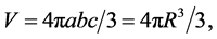 (1.6)
(1.6)
and we see that changes of  and
and  do not change the volume, only the shape of the ellipsoid.
In what follows, we will also consider the special case of spheroids. A spheroid is an ellipsoid with two equal semi-axes. We take . This means that we take
  in the formulas above so that
 (1.7)
(1.7)
and (1.4) becomes
 (1.8)
(1.8)
A spheroid is thus defined as the set of points that fulfill
 (1.9)
(1.9)
Here R is the (geometric) mean radius and  is a parameter that determines the shape in such a way that
  corresponds to a prolate spheroid,
  to a sphere, and
  to an oblate, or flattened, spheroid.
More familiar parameters used to define the shape of a spheroid are the ellipticity  and the eccentricity e. The ellipticity is defined by
 (1.10)
This is sometimes also called the (geometric) oblateness or the flattening (denoted f). Solving this equation, and expanding around , we have
 (1.11)
One notes that  is positive for oblate and negative for prolate spheroids respectively. The eccentricity
  is defined as the usual eccentricity of the ellipse that is the intersection of the spheroid and a plane containing the z-axis. One finds that
 (1.12)
gives the eccentricity of these ellipses in the oblate case. For the prolate case .
.
3. The Mass Distribution
Consider a non-rotating spherically symmetric body consisting of point particles with masses mi and position vectors
 . (1.13)
Assume that rotation induces a deviation of the positions so that the new positions,  , are given by
 . (1.14)
This implies that we assume that the elastic displacement field can be parameterized by the shape parameters  with non-rotating positions corresponding to
 . One notes that points r0 that obeyed
  i.e. were found on a sphere of radius
 , move to the surface given by
 (1.15)
The sphere is thus assumed to deform to an ellipsoid.
Assume that a body initially is spherically symmetric and has a mass density , where r is the ordinary distance from the center. It is tempting to assume that a natural deformation of the body when it starts to rotate is to a spheroidal shape in such a way that the originally spherical equidensity surfaces,
  , deform to similar spheroidal surfaces given by
 . Unfortunately this is an approximation for real bodies. For a density that increases towards the center, the ellipticity of the equidensity surfaces decrease with r, in a manner described by Clairaut’s equation, see [5] [7] [8] [18] . Note, however, that for a constant density, or a constant density with a central point mass, the assumption is not approximate, since any surface is an equidensity surface, only the shape of the outer surface matters.
Thus we now assume such a mass distribution. To be precise we assume that a mass M1 is distributed with constant density
 (1.16)
inside the surface,  , and that the point mass
  is at the center,
  , of the ellipsoid. The density
  is thus given by
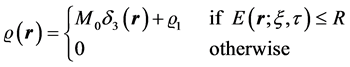 (1.17)
where  is the three-dimensional Dirac delta function.
4. Moments of Inertia and the Quadrupole Tensor
If we put mi for the masses of the particles, the inertia tensor of the body is given by
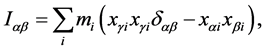 where we have put,
  and
and  is the usual Kronecker delta. The inertia tensor for the non-rotating body is diagonal with all diagonal elements equal and given by
 (1.18)
Here we have introduced the total mass,
 (1.19)
as well as the dimensionless radius of gyration . The square of this parameter,
  , also appears in the literature denoted
  (or
(or , or simply k) and is also called the moment of inertia coefficient.
We calculate the dimensionless moment of inertia  for the undeformed
  of Equation (1.17). Using Equation (1.18) and
  we find
 (1.20)
where  and Equation (1.16) has been used. This is the usual moment of inertia for a solid sphere of mass
 . This implies that
 (1.21)
is the squared (dimensionless) radius of gyration of the undeformed body. Note that  since the model can go between the limits of a point
  and a homogeneous sphere
 .
.
For the deformed body one gets, using (1.14),
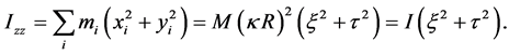 (1.22)
Izz is often denoted by C. For spheroids  the other moments of inertia become
 . For these one frequently finds the notation A, and B, respectively, in the literature.
The quadrupole tensor,  , is given in terms of the inertia tensor by
 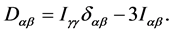 It is identically zero for the undeformed body and diagonal for the same axes as the inertia tensor. For the spheroidal
  body its components are given by
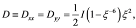 (1.23)
And  Thus
Thus  (or
(or ) is positive for oblate and negative for prolate shapes.
5. Potential and Hydrostatic Equilibrium
One measure of the oblate shape that is of great interest is the, so called, gravitational quadrupole J2. This dimensionless quantity, gives the deviation of the gravitational potential,  , outside the body, from the simple
  -dependence of spherically symmetric bodies. The first two terms in the multipole expansion of this potential are, see e.g. Stacey [19] ,
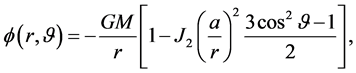 (1.24)
where  is the polar angle (colatitude) in spherical coordinates, M the total mass, and a the equatorial radius of the body. One can show [19] that J2 of formula (1.24) is given by
  Use of D given in (1.23), and
 , then gives
 (1.25)
for the quadrupole. Here we have also used  and Equation (1.12). Note that
  is independent of R, but directly proportional to the eccentricity squared.
Assuming the oblateness to be small, and due to hydrostatic equilibrium in the combined gravitational and centrifugal force fields, one can derive a formula connecting J2 with the angular velocity and the ellipticity. One uses that the shape of the surface is determined by the hydrostatic equilibrium equation
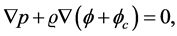 (1.26)
where p is pressure,  mass density, and
 (1.27)
is the potential of the centrifugal force in a system rotating with angular velocity ω about the z-axis. This means that the surface of the body must be an equipotential surface of . The constancy of
  on the surface of the body can be used to derive the approximate relationship
 (1.28)
[8] . Here we have introduced the ratio q of equatorial centrifugal to gravitational acceleration,
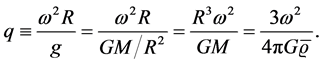 (1.29)
Here  is the mean density. Instead of q the notation m occurs in the literature, see Zharkov et al. [7] , who reserve q for the corresponding quantity with the equatorial radius a replacing the mean radius R (recall
 ). The advantage of the definition (1.29) is that it makes q independent of flattening. The relationship (1.28), is only valid to first order in small quantities, so here the difference does not matter, but we will go to higher order below, so take notice. This relationship between the three quantities q (or m),
  (or f), and J2, can thus be used to test the hypothesis of hydrostatic equilibrium empirically. This will be done below, using more exact results. For Jupiter and Saturn these will improve significantly on (1.28).
6. Rotational and Gravitational Energy
To study a rotating body, we go to the rotating system, and assume that all particles are affected by the centrifugal and gravitational potential energies. If the system is rotating rigidly about the z-axis with angular velocity vector  the potential energy of particle i in the centrifugal force field is
 . The total centrifugal potential energy of the body (system of particles) is
 (1.30)
This is the negative of the rotational kinetic energy. Using (1.22) we can write
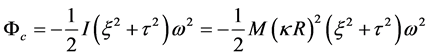 (1.31)
for the total potential energy of the particles in the centrifugal potential.
The gravitational potential from an ellipsoid (1.2), of constant density , at an interior point is [20]
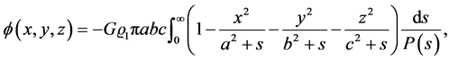 (1.32)
where . Since
  is the interaction energy of the homogeneous ellipsoid with a point particle of mass
  at the origin one finds the expression
 (1.33)
for this interaction energy. Here  and Equation (1.16) has been used.
An elementary calculation based on (1.32), see Landau and Lifshitz [21] , also shows that the gravitational self-energy of the ellipsoid is
 (1.34)
Use of the definitions (1.3) and the substitution  gives
gives
 (1.35)
If we define
 (1.36)
we find that the total gravitational energy of the mass distribution (1.17) is given by
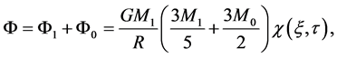 (1.37)
where . We define the constant
 , the dimensionless gravitational radius, through
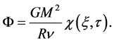 (1.38)
Comparing with (1.37) and using  together with the result (1.21), a small calculation reveals that the dimensionless gravitational radius,
  , is given by
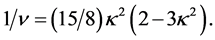 (1.39)
It is interesting to note that the gravitational energy of a density (1.17), with fixed mass M and radius R, is minimized for  (this is incidentally very close Earth’s value).
Using the definition (1.36), it is easy to find the Taylor expansion of  around
  This gives
 (1.40)
so the sphere really corresponds to a minimum in the gravitational energy. Higher order terms are easily generated by computer algebra programs, but we will not need them here. To study the behavior further away from the minimum one might use, instead of (1.36), an excellent Padé approximation of the ellipsoidal energy derived by Dankova and Rosensteel [22] . Near the spherical minimum, it is almost indistinguishable from the exact expression.
For spheroids we define
 (1.41)
to be the dimensionless gravitational potential energy. For  the integral in (1.36) can be found in terms of elementary functions. Several different alternative expressions exist and they are always different depending on whether
  is greater or less than unity. However, noting that,
  , the two expressions in
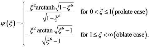 (1.42)
are equivalent and can be used for all . These are really the same real function if only the correct branch is chosen when passing through
 . Series expansion, of either alternative, around
  gives
gives
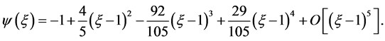 (1.43)
This function, which is shown in Figure 1, has the following properties. The prolate limit,  , of an infinite line is zero:
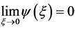 . The oblate limit,
  , an infinite circular disc, is also zero:
 .
.
The sphere  corresponds to a minimum of
  so that
 ,
,  , and
, and .
.
7. Minimizing the Energy
The total energy, U, of a static body (star or planet) will, apart from the centrifugal energy,  of Equation (1.31), and gravitational energy,
  of Equation (1.38), also consist of some volume dependent energy,
 . We can then write this total energy it in the form
 (1.44)s
Figure 1. The function  of equation Equation (1.42) which gives the dimensionless gravitational energy of a homogeneous spheroid with a central point mass. The minimum at
  corresponds to a sphere.
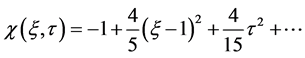
By minimizing this energy, we can find out whether a system tends to be triaxial or spheroidal. For small angular velocities the spheroidal case is known to be relevant [10] [22] . We thus put  here and get
 (1.45)
Using this we can find out if the body will be prolate or oblate and how this is affected by rotation. Since we concentrate on stars and planets surface forces and other neglected shape dependent forces are normally very small compared to the gravitational and centrifugal energies.
The equilibrium equations can be written
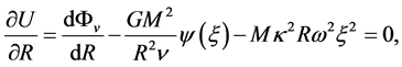 (1.46)
 (1.47)
where we have denoted differentiation by  with a prime. If we multiply the first equation by R and the second by
  and subtract we get, after rearrangement,
 (1.48)
This is essentially an equation of hydrostatic equilibrium. Note that it determines the equilibrium R-value with no direct reference to the angular velocity . The second equation, (1.47) can be written
 (1.49)
and this expresses a balance of the shape dependent part of the gravitational force with the centrifugal force. If we put
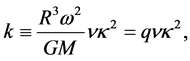 (1.50)
this turns into the concise expression
 (1.51)
Since  this will cause a shift of the shape from the spherical equilibrium, at
 , to
, to , as long as
 . Use of (1.39) shows that
 . (1.52)
The equilibrium  is thus entirely determined by q and the moment of inertia
 .
.
8. Finding the Position of the Minimum
To investigate Equation (1.51), we use the second variant for  in Equation (1.42) and get, after some algebra,
 (1.53)
This looks simpler if we introduce the new variable . Use of Equation (1.12) shows that
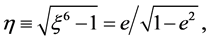 (1.54)
so that  can also be regarded as a function of the eccentricity
 . Now we get
 (1.55)
For the homogeneous case  and this formula, written in terms of the eccentricity by means of the identity,
  , is equivalent to the celebrated Maclaurin’s formula [10] from 1742.
Taylor expansion of the Maclaurin function around e = 0 only contains positive even powers of e. The coefficient of e6 vanishes so a very good approximation for this function is implied by
 (1.56)
The two term approximation is nearly perfect for all planetary e-values, see Figure 2. Saturn has maximum e = 0.43 and the absolute error at this value is 2 × 10⁻⁵ and the relative error is 4 × 10⁻⁴. The relative error even remains below 1% up to e = 0.75.
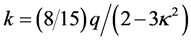
Using this approximation we must solve
 (1.57)
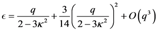
and solving this for e2 gives
 (1.58)
Use of Equation (1.25) gives . Insertion of this into (1.52) eliminates
  from
from . Some algebra then leads to the equation
 (1.59)
for q. This equation can be solved for J2 or for  to give
 (1.60)
 (1.61)
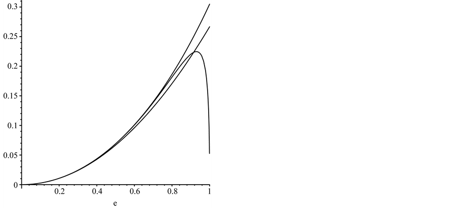
Figure 2. The Maclaurin function  with
with  compared to the approximations
  (lower curve) and
  (upper curve).
respectively. These results, together with
 (1.62)
 (1.63)
are thus more exact versions of Equation (1.28). Already the approximation , to the Maclaurin function, gives only a 3% error for Saturn, and simpler formulae, but use of these more exact versions removes all numerical considerations from the problem.
9. Theory versus Observational Data
Table 1 compares modern data with the predictions of Equations (1.59)-(1.63). Observed data for q,  , and J2 from Lodders and Fegeley [23] are given in the first (horizontal) row of data for each of the major rotating planets. In the same line e2 calculated from
  is then given. The last value in the row is the dimensionless moment of inertia
  as given by Lodders and Fegeley [23] . These values are based on calculation. For original sources the reader may consult The Planetary Scientist’s Companion by Lodders and Fegeley [23] .
For each pair of the values q, J2, and e2, in the first row, the third value is calculated using (1.59)-(1.61) and the results are displayed in the second row of data for each planet in Table 1.  is then found from Equation (1.63). For Jupiter and Saturn there is a third row of data in Table 1. This row is analogous to the second row except that the data are calculated from observational pairs of data using the first order formula (1.28) so that q is given by observational
  and J2 according to
 ,
,  is found directly from (1.28) using the observational q and J2, and so on. These rows illustrate the fact that the non-linear formulas of this work are more accurate than first order results, in spite of the point core approximation. Even for the Earth the first order formula gives discrepancies in the third digit.
Table 1 shows clearly that the observational data and theory are in reasonable agreement for the planets with the exception of Mars and Uranus. The perfect agreement for the Earth is probably due to the fact that the oblateness is determined from the shape of the geoid (the equipotential surface at sea-level). For Mars the disagreement may depend on the fact that oblateness is determined from geometrical shape rather than from the shape of an equipotential surface. Also, of course, the assumption of hydrostatic equilibrium may not be perfect for Mars. The problems with the Uranus data, and to some extent those for Neptune, are probably due to observational uncertainty.
10. Oblateness and Moment of Inertia
Instead of eliminating the moment of inertia (or mass ratio)  of Equation (1.21) from the equations as done above one can retain it and try to use observed data to get information about
 . Series expansion of Equation (1.55) with
  expressed in terms of appropriate variables gives
 (1.64)
for the flattening, or oblateness, expressed in terms of q and the dimensionless moment of inertia. For a homogeneous body  so
so  and the old Newtonian result,
  , is obtained, to first order. In the opposite (Roche) limit of dominating central mass
  and one finds
 .
.
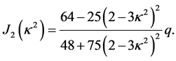
In a similar way we get from J2 of Equation (1.25) that
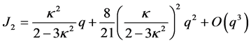 (1.65)
is the dimensionless quadrupole moment of the rotating body. For the homogeneous  body this implies
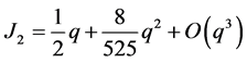 . In the opposite limit of
  one finds that J2 goes to zero.
Our results (1.64) and (1.65), to first order, are
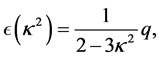 (1.66)
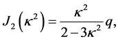 (1.67)
and imply that . These may be compared to similar expressions derived by G. H. Darwin using the Radau equation [8]
 (1.68)
 (1.69)
These two have the same values at , the homogeneous sphere, and the same derivatives with respect to
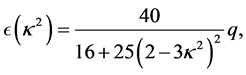
  at this point, as (1.66) and (1.67) respectively. The simple expressions (1.66) and (1.67), derived here, however, also have natural limits for
 , in contrast to e.g. (1.69), which becomes negative for
We now use Equation (1.25) i.e.  and Equation (1.61) for
  to calculate
  in terms of the observed q and J2. The last entry in the second row for each planet of Table 1 gives
 ,
,
 (1.70)
as calculated from observational, first row, q and J2. Since q and J2 are easier to measure accurately than flattening this should give more reliable values than using the observed ellipticity directly. In this way, one obtains information about the radial mass distribution in the interior of the planet from purely external data. The resulting  -values are given last in the second line for each planet in Table 1. The data obtained in this way are compared with published and tabulated
  -values for the planets (Lodders and Fegley [23] ). For Earth and Mars the agreement is reassuring. For the outer planets there is naturally a lot of uncertainty but at least the increasing trend from a minimum at Saturn is a common feature.
One problem with the outer planets is that the angular velocity is not constant. For a recent study of Saturn’s rotation, see Anderson and Schubert [24] . Also for the Sun, it is hard to decide what angular velocity,  , should be used to find q. Since these bodies have differential rotation some average must be used. There is a well-defined theoretical average angular velocity (Essén [25] ) but it is not directly observable. Once an average angular velocity has been selected for the Sun, one can use the present theory and a theoretical
  -value (0.059) to estimate the solar oblateness and J2. The definition of average angular velocity in [25] indicates that an angular velocity near the radius of gyration
  should be appropriate. The further assumption that angular velocity is constant on coaxial cylinder surfaces (Kippenhahn and Weigert [13] , Ulrich and Hawkins [26] ) indicates that an angular velocity near the poles of the Sun rather than equatorial angular velocity is relevant.
A handbook value [23] for the polar angular velocity of the Sun is . Use of this gives the q-value (1.15 × 10⁻⁵) in Table 1. The precise numbers are not important here. What is important is that, because of the small
 , an angular velocity near the pole rather than an equatorial angular velocity is used. Otherwise the flattening will be exaggerated. Use of
  and
and  from Lodders and Fegley [23] , together with formulas (1.66) and (1.67), gives the results in the top row of Table 1, that is,
  , and
, and . These values are, at least, of the same order of magnitude as the currently best motivated values [3] [4] [26] -[28] which are roughly
  and
and .
.
11. Small Oscillations near Equilibrium
We now wish to study the small amplitude motions of a gravitating rotating nearly spherical body. We wish to know how the radius R is affected by the rotation so we take R to denote the constant non-rotating equilibrium radius and let  be the variable radius.
  is thus a dimensionless variable which is equal to unity at the undeformed geometry. We parameterize the positions of the particles of the system as follows
 (1.71)
The  are then the non-rotating equilibrium dimensionless position coordinates of the particles. Equilibrium corresponds to
 ,
,  , see Section 2.
  is a dilatation (or radial pulsation) degree of freedom, while
  corresponds to spheroidal deformations and
  to triaxial deformations.
The velocities of the particles are
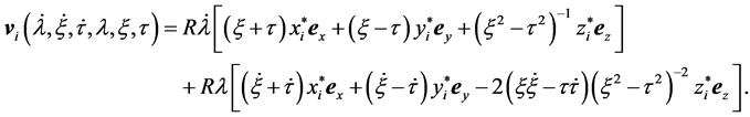 (1.72)
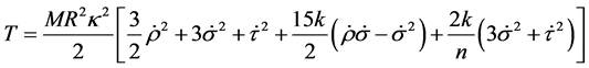
An elementary computation shows that the kinetic energy,  , becomes
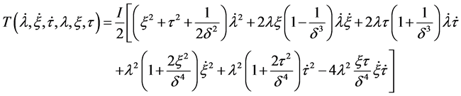 (1.73)
Here  and
and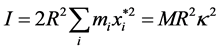 .
.
The potential energy is given in Equation (1.44). To get an explicit potential energy we must find some expression for the volume dependent (pressure) energy . As a model for this part of the energy we take the simple expression
 (1.74)
where we must take  if the corresponding force is to balance gravity and prevent collapse. Putting these together we thus find the total potential energy
 (1.75)
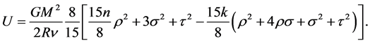
If we use the definition of k in Equation (1.50), we find the expression
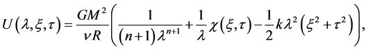 (1.76)
for the potential energy of the system.
Combining T of Equation (1.74) with U to the Lagrangian , we can get the dynamics of this three degree of freedom system exactly by finding and solving the Euler-Lagrange equations of the system. Here we will instead assume small oscillations and make a normal mode analysis. We first Taylor expand U to quadratic terms around
  and then solve for the zeroes of the first derivatives of this quadratic to get the position of the minimum. The result is
 (1.77)
 (1.78)
 (1.79)
We now introduce new variables,  through
 (1.80)
then, of course, . In the kinetic energy, we replace
  in the coefficients with the equilibrium positions
  and expand to first order in k. In the potential energy, we make the same replacement in the quadratic Taylor expansion, expand to first order in k and throw away constant terms. The result is that
 (1.81)
and that
 (1.82)
Only the degrees of freedom  and
and  are coupled and only when
 . For
. For , the spheroidal
  - mode and the triaxial
  -mode are degenerate (have the same frequency). The value
  is special since for that value all three modes have the same frequency.
For the  -mode pressure is restoring force in the contracting phase of the motion and gravity in the expanding phase. For the other two modes,
  ,
,  , gravity alone acts to restore the spherical minimum. If we put
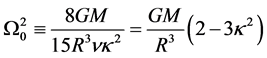 (1.83)
Equation (1.50) shows that , and Equation (1.57), with
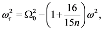
 , that
 . For
. For  we then get the approximate eigen frequencies
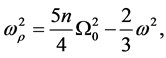 (1.84)
 (1.85)
 (1.86)
to first order in k. From this one easily finds the following first order results
 (1.87)
 (1.88)
 (1.89)
for the corresponding periods.
The free radial oscillation mode for the Earth is known [29] to have . This means that one can calculate n and find it to be n = 13.19 for the Earth. Since the equilibrium radius of the rotating Earth is
  Equation (1.78), and a small calculation, now shows that Earth’s mean radius is 863 m larger due to rotation compared to the non-rotating case. The fairly large n also shows that the g mode periods are essentially independent of n. For the Earth one finds that the
  -mode has period
 . Due to the rotational splitting, which is given by
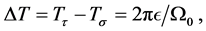 (1.90)
The  -mode is 17 seconds shorter. The longest observed free oscillation period of the Earth has period 53.8 min (see Udias [29] ). The main explanation for the discrepancy is probably that the model neglects elastic forces. Though not quantitatively reliable from this point of view, the model has the advantages of showing in a simple way how rotational splitting of the modes arises and the order of magnitude of such splittings.
12. Conclusion
The basic non-linearity of the problem of rotational flattening of a gravitationally bound body is illustrated by the fact that even the simplest conceivable model leads to a cubic equation [30] . Here some apparently new results relating to the classic theory of the figure of rotating bodies have been presented. The basic model, a point mass at the center of a homogeneous fluid, is characterized by their mass ratio, and interpolates between the limits of an ellipsoidal homogeneous fluid and a body dominated by a small central mass concentration. It allows simple analytic treatment but is still flexible enough to correctly describe the essential hydrostatics of real rotating planets as well as stars. Such models are always useful, especially when one wishes to analyze, compare, and understand large numbers of observational data. In spite of the simplicity, there is no perturbation order to which the results are valid. The nonlinearity of the basic equations can be retained. To be more precise, Equation (1.56) shows that the formulas are valid to seventh order in the eccentricity (within the basic model with its simplified mass distribution). As demonstrated by the numerical experiments on Jupiter and Saturn data, this is essential. In fact, Table 1 indicates that the geometric oblateness of the surface equipotential surface of Mars and Uranus determined from observed q and J2 values using (1.61) probably are more reliable than current observational data. Finally the dynamics of the model reveals the essentials of the coupling and rotational splitting of the most basic free oscillations of a planet without recourse to expansion in spherical harmonics.
Acknowledgements
Constructive comments from Dr. John D. Anderson on a previous version of this manuscript are gratefully acknowledged.
References
- Todhunter, I. (1873) A History of the Mathematical Theories of Attraction and the Figure of the Earth. Macmillan and Company, London. (Reprinted: Dover Publications, New York, 1962)
- Will, C.M. (1993) Theory and Experiment in Gravitational Physics. Cambridge University Press, Cambridge. http://dx.doi.org/10.1017/CBO9780511564246
- Godier, S. and Rozelot, J.-P. (1999) Quadrupole Moment of the Sun. Gravitational and Rotational Potentials. Astronomy & Astrophysics, 350, 310-317.
- Laskar, J. (1999) The Limits of Earth Orbital Calculations for Geological Timescale Use. Philosophical Transactions of the Royal Society A, 357, 1735-1759. http://dx.doi.org/10.1098/rsta.1999.0399
- Jeffreys, H. (1962) The Earth, Its Origin History and Physical Constitution. 4th Edition, Cambridge University Press, Cambridge.
- Jardetzky, W.S. (1958) Theories of Figures of Celestial Bodies. Interscience, New York.
- Zharkov, V.N. and Trubitsyn, V.P. (Editor Hubbard, W.B.) (1978) Physics of Planetary Interiors. Pachart Publishing House, Tuscon.
- Cook, A.H. (1980) Interiors of the Planets. Cambridge University Press, Cambridge. http://dx.doi.org/10.1017/CBO9780511721748
- Moritz, H. (1990) The Figure of the Earth. Wichmann, Karlsruhe.
- Chandrasekhar, S. (1969) Ellipsoidal Figures of Equilibrium. Yale University Press, New Haven and London.
- Murray, C.D. and Dermott, S.F. (1999) Solar System Dynamics. Cambridge University Press, Cambridge.
- Kaula, W.M. (2000) Theory of Satellite Geodesy. Dover, Mineola.
- Kippenhahn, R. and Weigert, A. (1990) Stellar Structure and Evolution. Springer-Verlag, Berlin. http://dx.doi.org/10.1007/978-3-642-61523-8
- Hubbard, W.B. and Anderson, J.D. (1978) Possible Flyby Measurements of Galilean Satellite Interior Structure. Icarus, 33, 336-341. http://dx.doi.org/10.1016/0019-1035(78)90153-7
- Dermott, S.F. and Thomas, P.C. (1988) The Shape and Internal Structure of Mimas. Icarus, 73, 25-65. http://dx.doi.org/10.1016/0019-1035(88)90084-X
- Abad, S., Pacheco, A.F. and Sañudo, J. (1995) Variational Methods to Calculate the Hydrostatic Structure of Rotating Planets. Geophysical Journal International, 122, 953-960. http://dx.doi.org/10.1111/j.1365-246X.1995.tb06848.x
- Denis, C., Tomecka-Suchon, S., Rogister, Y. and Amalvict, M. (2000) Comment on “Variational Methods to Calculate the Hydrostatic Structure of Rotating Planets” by S. Abad, A. F. Pacheco, and J. Sa-udo. Geophysical Journal International, 143, 985-986. http://dx.doi.org/10.1046/j.1365-246X.2000.00294.x
- Denis, C., Amalvict, M., Rogister, Y. and Tomecka-Suchon, S. (1998) Methods for Computing Internal Flattening, with Applications to the Earth’s Structure and Geodynamics. Geophysical Journal International, 132, 603-642. http://dx.doi.org/10.1046/j.1365-246X.1998.00449.x
- Stacey, F.D. (1969) Physics of the Earth. John Wiley, New York.
- MacMillan, W.D. (1958) The Theory of the Potential. Dover, New York.
- Landau, L. and Lifshitz, E.M. (1975) The Classical Theory of Fields. 4th Edition, Pergamon, Oxford.
- Dankova, Ts. and Rosensteel, G. (1998) Triaxial Bifurcations of Rapidly Rotating Spheroids. American Journal of Physics, 66, 1095-1100. http://dx.doi.org/10.1119/1.19050
- Lodders, K. and Fegley Jr., B. (1998) The Planetary Scientist’s Companion. Oxford University Press, New York.
- Anderson, J.D. and Schubert, G. (2007) Saturn’s Gravitational Field, Internal Rotation, and Interior Structure. Science, 317, 1384-1387. http://dx.doi.org/10.1126/science.1144835
- Essén, H. (1993) Average Angular Velocity. European Journal of Physics, 14, 201-205. http://dx.doi.org/10.1088/0143-0807/14/5/002
- Ulrich, R.K. and Hawkins, G.W. (1981) The Solar Gravitational Figure—J2 and J4. The Astrophysical Journal, 246, 985-988. http://dx.doi.org/10.1086/158992
- Paterno, L., Sofia, S. and Di Mauro, M.P. (1996) The Rotation of the Sun’s Core. Astronomy & Astrophysics, 314, 940-946.
- Lydon, T.J. and Sofia, S. (1996) A Measurement of the Shape of the Solar Disc (the Solar Quadrupole Moment, the Solar Octopole Moment, and the Advance of the Perihelion of the Planet Mercury). Physical Review Letters, 76, 177179. http://dx.doi.org/10.1103/PhysRevLett.76.177
- Udías, A. (1999) Principles of Seismology. Cambridge University Press, Cambridge.
- Essén, H. (1996) A Simple Mechanical Model for the Shape of the Earth. European Journal of Physics, 17, 131-135. http://dx.doi.org/10.1088/0143-0807/17/3/006.