International Journal of Geosciences
Vol.5 No.4(2014), Article ID:45041,10 pages
DOI:10.4236/ijg.2014.54035
Model Simulation of Artificial Heating of the Daytime High-Latitude F-Region Ionosphere by Powerful High-Frequency Radio Waves
Galina Mingaleva, Victor Mingalev
Polar Geophysical Institute, Kola Scientific Center of the Russian Academy of Sciences, Apatity, Murmansk Oblast, Russia
Email: mingalev@pgia.ru
Copyright © 2014 by authors and Scientific Research Publishing Inc.
This work is licensed under the Creative Commons Attribution International License (CC BY).
http://creativecommons.org/licenses/by/4.0/


Received 18 February 2014; revised 16 March 2014; accepted 12 April 2014
Abstract
The large-scale disturbance of the spatial structure of the daytime high-latitude F-region ionosphere, caused by powerful high-frequency radio waves, pumped into the ionosphere by a groundbased ionospheric heater, is studied with the help of the numerical simulation. The mathematical model of the high-latitude ionosphere, developed earlier in the Polar Geophysical Institute, is utilized. The mathematical model takes into account the drift of the ionospheric plasma, strong magnetization of the plasma at F-layer altitudes, geomagnetic field declination, and effect of powerful high-frequency radio waves. The distributions of the ionospheric parameters were calculated on condition that an ionospheric heater, situated at the point with geographic coordinates of the HF heating facility near Tromso, Scandinavia, has been operated, with the ionospheric heater being located on the day side of the Earth. The results of the numerical simulation indicate that artificial heating of the ionosphere by powerful high-frequency waves ought to influence noticeably on the spatial structure of the daytime high-latitude F-region ionosphere in the vicinity of the ionospheric heater.
Keywords: High-Latitude Ionosphere, Active Experiments, Modeling and Forecasting, Plasma Temperature and Density

1. Introduction
For the investigation of the ionospheric plasma’s properties, experiments with high-power, high-frequency (HF) radio waves, pumped into the ionosphere by a ground-based ionospheric heater, were successfully used during the last four decades. For this investigation, some high-power radio wave heaters have been built over the world. Initially, these heaters were built in the mid-latitudes (Platteville, Arecibo, Nizhny Novgorod, etc.). Later, some ionospheric heaters were applied for investigation of the high-latitude ionosphere owing to their location in the high-latitudes, namely, near Monchegorsk, Kola Peninsula, near Tromso, Scandinavia, near Fairbanks, Alaska, near Gakona, Alaska, and near Longyearbyen, Svalbard. Experiments with high-power, high-frequency radio waves indicate that these radio waves cause the variety of physical processes in the ionospheric plasma. Some of such processes can result in the large-scale disturbances of the height profiles of the ionospheric parameters at F-layer altitudes (above approximately 150 km). The experiments indicated that powerful HF waves can produce significant large-scale variations in the electron temperatures and densities at F-layer altitudes [1] -[21] .
To investigate the physical mechanisms responsible for the disturbances of the F-region ionosphere by a powerful HF wave, mathematical models may be utilized. However, to date very few mathematical models of the F-region ionosphere, which can be affected by a powerful HF wave, have been developed. One of such mathematical models has been developed in the Polar Geophysical Institute (PGI) [22] . This model has been used to simulate the influence of the power, frequency, and modulation regime of the HF waves on the expected response of the ionospheric parameters at F-layer altitudes to HF heating [23] -[27] .
The purpose of the present paper is to examine how high-power high-frequency radio waves, pumped into the high-latitude ionosphere, influence on the large-scale ionospheric parameters distributions in the horizontal directions at F-layer altitudes. The distributions of the ionospheric parameters were calculated on condition that an ionospheric heater, situated at the point with geographic coordinates of the HF heating facility near Tromso, Scandinavia, has been operated, with the ionospheric heater being located on the day side of the Earth on the magnetic meridian of 15.00 MLT. The mathematical model of the high-latitude ionosphere, developed earlier in the PGI, which takes into account the effect of powerful high-frequency radio waves, is utilized in this study.
2. Mathematical Model
In the present study, to investigate the large-scale disturbances of the spatial structure of the high-latitude F-region ionosphere, caused by powerful HF radio waves, pumped into the ionosphere by a ground-based ionospheric heater, the mathematical model is utilized. In essence, the utilized model is the modified version of the mathematical model of the convecting high-latitude ionosphere, developed earlier by Mingaleva and Mingalev [28] [29] .
The latter model produces three-dimensional distributions of the electron density, positive ion velocity, and ion and electron temperatures. It encompasses the ionosphere above 36˚ magnetic latitude and at distances between 100 and 700 km from the Earth along the magnetic field line for one complete day. The applied numerical model takes into consideration the strong magnetization of the plasma at F-layer altitudes and the attachment of the charged particles of the F-region ionosphere to the magnetic field lines. As a consequence, the F-layer ionosphere plasma drift in the direction perpendicular to the magnetic field B is strongly affected by the electric field E and follows E ´ B convection paths (or the flow trajectories). In the model calculations, a part of the magnetic field tube of the ionospheric plasma is considered at distances between 100 - 700 km from the Earth along the magnetic field line. The temporal history is traced of the ionospheric plasma included in this part of the magnetic field tube moving along the flow trajectory through a neutral atmosphere. By tracing many field tubes of plasma along a set of flow trajectories, we can construct three-dimensional distributions of ionospheric quantities.
As a consequence of the strong magnetization of plasma at F-layer altitudes, its motion may be separated into two flows: the first, plasma flow parallel to the magnetic field; the second, plasma drift in the direction perpendicular to the magnetic field. The parallel plasma flow in the considered part of the magnetic field tube is described by the system of transport equations, which consists of the continuity equation, the equation of motion for ion gas, and heat conduction equations for ion and electron gases. These equations in the reference frame, convecting together with a field tube of plasma, whose axis h is directed upwards along the magnetic field line, may be written as follows:
 (1)
(1)
 (2)
(2)
 (3)
(3)
 (4)
(4)
where N is the O+ ion number density (which is assumed to be equal to the electron density at the F-layer altitudes); Vi is the parallel (to the magnetic field) component of the positive ion velocity; q is the photoionization rate; qe is the production rate due to auroral electron bombardment; qp is the production rate due to auroral proton bombardment; l is the positive ion loss rate (taking into account the chemical reactions)

mi is the positive ion mass; k is Boltzmann’s constant; Ti
and Te are the ion and electron temperatures, respectively;
g is the acceleration due to gravity; I is the magnetic field dip angle; 1/ is the collision frequency between ion and neutral particles of type n; Un
is the parallel component of velocity of neutral particles of type n;
is the collision frequency between ion and neutral particles of type n; Un
is the parallel component of velocity of neutral particles of type n;
 ; Ve is the parallel component of electron
velocity (which is determined from the equation for parallel current);
; Ve is the parallel component of electron
velocity (which is determined from the equation for parallel current);
 is the ion viscosity coefficient;
 and
and
 are the ion and electron thermal conductivity coefficients; Q, Qe, Qp
and Qf are the electron heating rates due to photoionization, auroral
electron bombardment, auroral proton bombardment, and HF heating, respectively;
Lr, Lv, Le and Lf are the electron cooling
rates due to rotational excitation of molecules O2 and N2,
vibrational excitation of molecules O2 and N2, electronic
excitation of atoms O, and fine structure excitation of atoms O, respectively.
are the ion and electron thermal conductivity coefficients; Q, Qe, Qp
and Qf are the electron heating rates due to photoionization, auroral
electron bombardment, auroral proton bombardment, and HF heating, respectively;
Lr, Lv, Le and Lf are the electron cooling
rates due to rotational excitation of molecules O2 and N2,
vibrational excitation of molecules O2 and N2, electronic
excitation of atoms O, and fine structure excitation of atoms O, respectively.
The quantities on the right-hand sides of Equations (3) and (4), denoted by Pab, describe the type a particles energy change rates as a result of elastic collisions with particles of type b, with large drift velocity differences having been taken into account. Thus, the quantities Pab contain the frictional heating produced by electric fields and thermospheric winds. Concrete expressions of the model parameters that appear in the Equations (1)-(4) are the same as in the papers by Mingaleva and Mingalev [28] [29] .
The plasma drift in the direction perpendicular to the magnetic field coincides with the motion of the magnetic field tube along the flow trajectory which may be obtained using the plasma convection pattern. The use of plasma convection pattern allows us not only to obtain the configurations of the flow trajectories but also to calculate the plasma drift velocity along them at an F-layer altitude. It is known that the convection trajectories, around which the magnetic field tubes are carried over the high-latitude region, are closed for a steady convection pattern. For each flow trajectory, we obtain variations of ionospheric quantities with time (along the flow trajectory), that is, the profiles against distance from the Earth along the geomagnetic field line of the electron density, positive ion velocity, and electron and ion temperatures are obtained by solving the system of transport equations of ionospheric plasma, described above. These profiles result in two-dimensional steady distributions of ionospheric quantities along the each flow trajectory. By tracing many field tubes of plasma along a set of convection trajectories, we can construct three-dimensional distributions of ionospheric quantities. The neutral atmosphere composition, input parameters of the model, numerical method, and boundary conditions were in detail described in the studies by Mingaleva and Mingalev [28] [29] .
As pointed out previously, the model, utilized in the present study, is the modified version of the mathematical model of the convecting high-latitude ionosphere, described briefly above. The modification consists in taking into account the heating mechanism, caused by the action of the powerful HF radio waves. Due to this heating mechanism, the energy absorption of a powerful HF wave in the ionosphere can take place. It can be noticed that only part of the effective radiated power (ERP) is absorbed by the ionospheric plasma, this part is referred to as the effective absorbed power (EAP). It is known that the EAP is connected with the effective radiated power (ERP) by the formula
 (5)
(5)
where η is the coefficient characterizing the fraction of the energy of the powerful HF wave deposited in the ambient electron gas and lost for its heating. In the concrete ionospheric heating experiment, the value of the coefficient η is not known exactly. Moreover, distinct high-power radio wave heaters can provide different values of the ERP. Therefore, in various ionospheric heating experiments, the values of the EAP may be different. Therefore, the EAP is chosen as an input parameter of the mathematical model.
The model, utilized in the present study, takes into account the following heating mechanism, caused by the action of the powerful HF radio waves. The absorption of the heater wave energy is supposed to give rise to the formation of field-aligned plasma irregularities on a wide range of spatial scales. In particular, short-scale field-aligned irregularities are excited in the electron hybrid resonance region. These irregularities are responsible for the anomalous absorption of the electromagnetic heating wave (pump) passing through the instability region and cause anomalous heating of the plasma. The rate of this anomalous heating is denoted by Qf and included in the heat conduction equation for electron gas, Equation (4). The concrete expression to the Qf, containing the EAP, was taken from the study by Blaunshtein et al. [30] . This expression was in detail reproduced in the studies by Mingaleva and Mingalev [22] and Mingaleva et al. [27] . It can be noted that this rate of anomalous heating is directly proportional to the EAP. Consequently, a necessity of knowledge of the precise value of the coefficient η, present in Equation (5), is absent. In the utilized model, the EAP is the input parameter of the model. The utilized expression of the rate of anomalous heating, in spite of its simplicity, allows us to evaluate approximately the influence of artificial heating of the ionosphere on the expected large-scale F-region modification.
In the present study, the electric field distribution, which is the combination of the pattern B of the empirical models of high-latitude electric fields of Heppner [31] and the empirical model of ionospheric electric fields at middle latitudes, developed by Richmond [32] and Richmond et al. [33] , is utilized. The utilized electric field distribution is a steady non-substorm convection model (Figure 1). Using this convection model, we calculate the plasma drift velocity along the convection trajectories, which intersect the F-layer volume illuminated by an ionospheric heater situated at the point with geographic coordinates of the HF heating facility near Tromso, Scandinavia. For these convection trajectories, we obtain variations of profiles against distance from the Earth along the geomagnetic field line of the ionospheric quantities with time (along the trajectory) by solving the system of transport equations. These profiles may be used for the construction of two-dimensional distributions of ionospheric quantities along the each flow trajectory. By taking a set of flow trajectories and using these two-dimensional distributions along the each convection trajectory, we can construct three-dimensional distributions of ionospheric quantities, modified by the action of the ionospheric heater.
In this study, the spatial configuration of the electron and proton precipitation zones as well as intensities and average energies of the precipitating electrons and protons were chosen as consistent with the statistical model of Hardy et al. [34] . The numerical method, boundary conditions, neutral atmosphere composition, thermospheric wind pattern, and input parameters of the model were in detail described in the studies by Mingaleva and Mingalev [22] , [28] , and [29] .
3. Presentation and Discussion of Results
Different combinations of the solar cycle, geomagnetic activity level, and season may be described by the utilized mathematical model. In the present study, the calculations are performed for autumn (5 November) and not high solar activity conditions (F10.7 = 110) under low geomagnetic activity (Kp = 0). In the present study, the calculations were made for two distinct cases. For the first case, we simulated the distributions of the ionospheric parameters under natural conditions without a powerful high-frequency wave effect. For the second case, the distributions of the ionospheric parameters were calculated on condition that an ionospheric heater, situated at the point with geographic coordinates of the HF heating facility near Tromso, Scandinavia, has been operated, with the ionospheric heater being located on the day side of the Earth on the magnetic meridian of 15.00 MLT (Figure 1).
For the second case, firstly, we made a series of calculations to choose the wave frequency which provides the maximal effect of HF heating on the electron concentration at the levels near to the F2-layer peak, that is, the most effective frequency for the large-scale F2-layer modification, feff, [25] . It was found that this most effective frequency is 4.9 MHz on condition that the maximal value of the effective absorbed power (EAP) is equal to 30 MW which is quite attainable for the heating facility near Tromso.
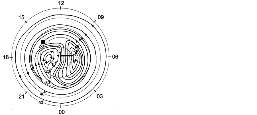
Figure 1.
Plasma convection trajectories derived from the combination of the pattern B of
the empirical convection models at polar latitudes of Heppner [31] and the empirical
model of ionospheric electric fields at middle latitudes, developed by Richmond
[32] and Richmond et al. [33] . Trajectories are depicted in the fixed sun-earth
reference frame. Magnetic local time (MLT) and magnetic colatitude
 are indicated on the plot. The arrows indicate the direction of convection flows.
The initial location of the ionospheric heater is indicated by the black square.
are indicated on the plot. The arrows indicate the direction of convection flows.
The initial location of the ionospheric heater is indicated by the black square.
Secondly, calculations were carried out, using the pointed out values of the feff and EAP, to study how the HF radio waves affect the large-scale high-latitude F-layer modification. The ionospheric heater was supposed to operate during the period of 435 seconds.
The results of simulations are presented in Figures 2-6. Results of simulation indicate that a great energy input from the powerful HF wave arises at the level, where the wave frequency is close to the frequency of the electron hybrid resonance, when the ionospheric heater is turned on and operates. As a consequence, the electron temperature can increase considerably (Figure 2). The increase in the electron temperature results in a visible decrease in the electron concentration profile at the levels near to the F2-layer peak (Figure 3). In particular, the powerful HF waves lead to the decrease of 24% in electron concentration at the level of the F2-layer peak.
After turning off of the heater, the electron temperature decreases due to elastic and inelastic collisions between electrons and other particles of ionospheric plasma, and a period of recovery comes.
In the model calculations, it was assumed that the ionospheric heater provides a beam width of 14.5˚ (such as the beam width of the ionospheric high-frequency heating facility near Tromce, Scandinavia [35] ). Therefore, the diameter of the illuminated region is approximately 88 km at 300 km altitude. As a consequence of the convection of the ionospheric plasma at F-layer altitudes, the volume of plasma, disturbed by a powerful HF wave, can abandon the region illuminated by an ionospheric heater. Therefore, the horizontal section of disturbed region at F-layer altitudes can differ from the horizontal section of the region illuminated by the heater.
Let us consider the simulated spatial distributions of the ionospheric parameters. These distributions are presented in Figures 4-6. The simulation results, obtained under natural conditions without artificial heating, contain various large-scale inhomogeneous structures characteristic for the high-latitude ionosphere. The electron concentration distributions contain the well-known tongue of ionization, extended from the local noon side of the Earth across the polar cap to the night side, auroral ionization peak, and main ionospheric trough on the night side of the Earth (Figure 5 and Figure 6). It can be seen that the electron temperature hot spots are formed in the main ionospheric trough in the dawn and dusk sectors (Figure 4).
The simulation results, obtained on condition that the ionospheric heater has been operated during the period of 435 seconds, indicate that the electron temperature hot spot is formed on the day side in the vicinity of the
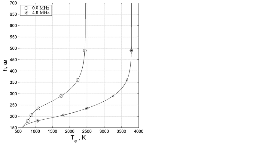
Figure 2. Profiles of the electron temperature versus distance from the Earth along the geomagnetic field line, situated in the illuminated region, obtained under natural conditions without artificial heating (left-hand curve) and disturbed by the heater at the moment of 435 seconds after turn on (righthand curve).
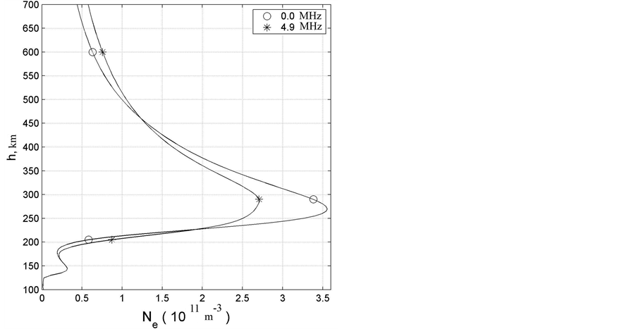
Figure 3. Profiles of the electron concentration versus distance from the Earth along the geomagnetic field line, situated in the illuminated region, obtained under natural conditions without artificial heating (marked by the symbol ○) and disturbed by the heater at the moment of 435 seconds after turn on (marked by the symbol *).
location of the ionospheric heater (Figure 4). Inside this hot spot, the electron temperature increases for some hundreds of degrees. Moreover, the electron concentration cavity is formed on the day side in the vicinity of the
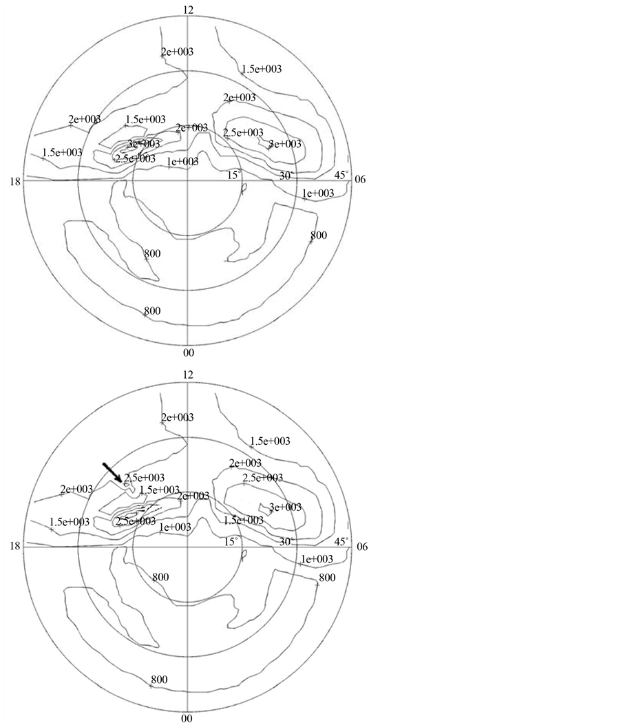
Figure 4. Simulated distributions of the electron temperature (K) at level of 280 km obtained under natural conditions without artificial heating (top panel) and obtained on condition that the ionospheric heater has been operated during the period of approximately seven minutes (bottom panel). The electron temperature hot spot, created artificially, is indicated by black pointer at the bottom panel.
location of the ionospheric heater (Figure 5 and Figure 6). Inside this cavity, powerful HF waves lead to a decrease of about 20% in the electron concentration at the level of the F2-layer peak.
The simulation results indicate that the cross sections of the artificial electron temperature hot spot and artificial electron concentration cavity have dimensions of about 90 - 150 km in the horizontal directions at the levels
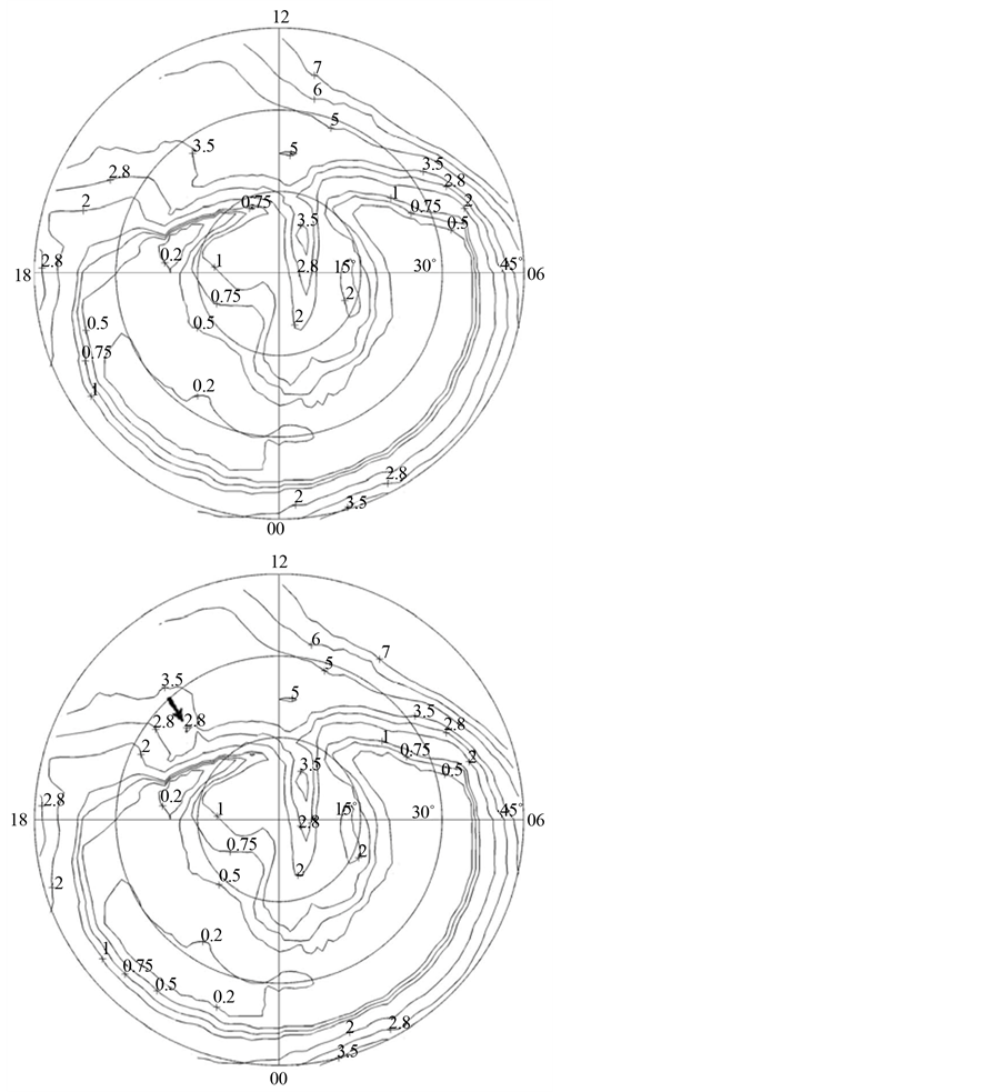
Figure 5. Simulated distributions of the electron concentration (in units of 1011 m−3) at level of 280 km obtained under natural conditions without artificial heating (top panel) and obtained on condition that the ionospheric heater has been operated during the period of approximately seven minutes (bottom panel). The electron concentration cavity, created artificially, is indicated by black pointer at the bottom panel.
of the F layer (Figures 4-6). These dimensions do not coincide with the horizontal section of the region, illuminated by the heater, due to the convection of the ionospheric plasma.
It is seen that these dimensions are much less than the horizontal sizes of the natural large-scale inhomogeneous structures characteristic for the high-latitude ionosphere, in particular, of the natural electron temperature hot spots and main ionospheric trough. The dimension of the artificial electron concentration cavity in the direction of the magnetic field line is about some hundreds of kilometers (Figure 6).
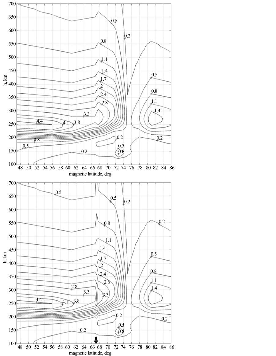
Figure 6. Simulated distributions of the electron concentration (in units of 1011 m−3) in the magnetic meridian plane, lying across the ionospheric heater, obtained under natural conditions without artificial heating (top panel) and obtained on condition that the ionospheric heater has been operated during the period of approximately seven minutes (bottom panel). The location of the heater is indicated by the black pointer at the bottom panel.
It can be noticed that the investigation, analogous to that carried out in the present work, has been fulfilled in the study by Mingaleva and Mingalev [36] . In this study, the distributions of the ionospheric parameters were calculated on condition that the ionospheric heater, situated at the point with geographic coordinates of the HF heating facility near Tromso, Scandinavia, has been operated during the period of five minutes, with the heater being located on the night side of the Earth on the magnetic meridian of 01.20 MLT. In this study, the most effective frequency equal to 2.6 MHz and the effective absorbed power (EAP) equal to 30 MW were used. The results of simulation, obtained for the night side of the Earth, indicated that the electron temperature hot spot was formed on the night side in the vicinity of the location of the ionospheric heater, with the electron temperature having increased for some thousands of degrees inside this hot spot. Moreover, the electron concentration cavity was formed on the night side in the vicinity of the location of the ionospheric heater, with the electron concentration having decreased for about 40% at the level of the F2-layer peak inside this cavity.
It is seen that the variations of the electron temperature and electron concentration, caused by the action of the HF heating and obtained in the present study for daytime conditions, are less than those, obtained for nighttime conditions in the study of Mingaleva and Mingalev [36] . This peculiarity is conditioned by the different values of the electron temperature and electron concentration in the daytime and nocturnal high-latitude F-region ionosphere under natural conditions (top panels of Figure 4 and Figure 5). The more the values of the electron temperature and electron concentration are, the less their relative variations, caused by artificial heating, ought to be.
It turned out that the cross sections of the artificial electron temperature hot spot and artificial electron concentration cavity, obtained for daytime and nighttime conditions, ought to be approximately equal.
4. Conclusions
To calculate three-dimensional distributions of ionospheric parameters in the high-latitude F layer, modified by the action of the ionospheric high-frequency heating facility, situated at the point with geographic coordinates of the HF heating facility near Tromso, Scandinavia, the mathematical model of the high-latitude ionosphere, developed earlier in the PGI, was utilized. The model is based on numerical solution of the system of transport equations, which consists of the continuity equation, equation of motion for ion gas, and heat conduction equations for ion and electron gases. The equations provide for the direct and resonantly scattered EUV solar radiation, energy-dependent chemical reactions, frictional force between ions and neutrals, accelerational and viscous forces of ion gas, thermal conductions of electron and ion gases, heating due to ion-neutral friction, Joule heating, heating due to solar EUV photons, heating caused by the action of the powerful HF radio waves, and electron energy losses due to elastic and inelastic collisions. The model takes into account the magnetization of the plasma at F-layer altitudes, drift of the ionospheric plasma, geomagnetic field inclination, and effect of powerful high-frequency radio waves.
Firstly, we simulated the distributions of the ionospheric parameters under natural conditions without a powerful high-frequency wave effect. These distributions have reproduced the remarkable natural features of the high-latitude ionosphere such as the tongue of ionization, main ionospheric trough, auroral ionization peak, and electron temperature hot spots in the morning and evening sectors of the main ionospheric trough.
Secondly, the distributions of the ionospheric parameters were calculated on condition that the ionospheric heater has been operated during the period of 435 seconds, using the most effective frequency for the large-scale F2-layer modification, with the heater being located on the day side of the Earth on the magnetic meridian of 15.00 MLT. These distributions, in addition to the natural features of the high-latitude ionosphere, contain the artificial electron temperature hot spot formed on the day side in the vicinity of the location of the ionospheric heater. Inside this hot spot, the electron temperature increases for some hundreds of degrees. Moreover, the artificial electron concentration cavity is formed on the day side in the vicinity of the location of the ionospheric heater. Inside this cavity, powerful HF waves lead to a decrease of about 20% in the electron concentration at the level of the F2-layer peak. The cross sections of the electron temperature hot spot and artificial electron concentration cavity have dimensions of about 100 - 150 km in the horizontal directions at the levels of the F layer. The artificial electron concentration cavity is stretched in the direction of the magnetic field line for some hundreds of kilometers.
The relative variations of the electron temperature and electron concentration, caused by the action of the HF heating and obtained in the present study for daytime conditions, are less than those, obtained for nighttime conditions in the study of Mingaleva and Mingalev [36] . The cross sections of the artificial electron temperature hot spot and artificial electron concentration cavity, obtained for daytime and nighttime conditions, ought to be approximately equal.
Acknowledgements
This work was partly supported by Grant No. 13-01-00063 from the Russian Foundation for Basic Research.
References
- Gordon, W.E. and Carlson, H.C. (1974) Arecibo Heating Experiments. Radio Science, 9, 1041-1047. http://dx.doi.org/10.1029/RS009i011p01041
- Utlaut, W.F. and Violette, E.J. (1974) A Summary of Vertical Incidence Radio Observations of Ionospheric Modification. Radio Science, 9, 895-903. http://dx.doi.org/10.1029/RS009i011p00895
- Kapustin, I.N., Pertsovskii, R.A., Vasil’ev, A.N., Smirnov, V.S., Raspopov, O.M., Solov’eva, L.E., Ul’yanchenko, A.A., Arykov, A.A. and Galachova, N.V. (1977) Generation of Radiation at Combination Frequencies in the Region of the Auroral Electric Jet. JETP Letters, 25, 228-231.
- Mantas, G.P., Carlson, H.C. and La Hoz, C.H. (1981) Thermal Response of F-Region Ionosphere in Artificial Modification Experiments by HF Radio Waves. Journal of Geophysical Research, 86, 561-574. http://dx.doi.org/10.1029/JA086iA02p00561
- Stubbe, P. and Kopka, H. (1983) Summary of Results Obtained with the Tromso Heating Facility. Radio Science, 18, 831-834. http://dx.doi.org/10.1029/RS018i006p00831
- Jones, T.B., Robinson, T.R., Stubbe, P. and Kopka, H. (1986) EISCAT Observations of the Heated Ionosphere. Journal of Atmospheric and Terrestrial Physics, 48, 1027-1035. http://dx.doi.org/10.1016/0021-9169(86)90074-7
- Djuth, F.T., Thide, B., Ierkic, H.M. and Sulzer, M.P. (1987) Large F-Region Electron-Temperature Enhancements Generated by High-Power HF Radio Waves. Geophysical Research Letters, 14, 953-956. http://dx.doi.org/10.1029/GL014i009p00953
- Duncan, L.M., Sheerin, J.P. and Behnke, R.A. (1988) Observations of Ionospheric Cavities Generated by High-Power Radio Waves. Physical Review Letters, 61, 239-242. http://dx.doi.org/10.1103/PhysRevLett.61.239
- Hansen, J.D., Morales, G.J., Duncan, L.M. and Dimonte, G. (1992) Large-Scale HF-Induced Ionospheric Modification: Experiments. Journal of Geophysical Research, 97, 113-122. http://dx.doi.org/10.1029/91JA02403
- Mantas, G.P. (1994) Large 6300-Å Airglow Intensity Enhancements Observed in Ionosphere Heating Experiments Are Exited by Thermal Electrons. Journal of Geophysical Research, 99, 8993-9002. http://dx.doi.org/10.1029/94JA00347
- Honary, F., Stocker, A.J., Robinson, T.R., Jones, T.B. and Stubbe, P. (1995) Ionospheric Plasma Response to HF Radio Waves Operating at Frequencies Close to the Third Harmonic of the Electron Gyrofrequency. Journal of Geophysical Research, 100, 21489-21501. http://dx.doi.org/10.1029/95JA02098
- Robinson, T.R., Honary, F., Stocker, A.J., Jones, T.B. and Stubbe, P. (1996) First EISCAT Observations of the Modification of F-Region Electron Temperatures during RF Heating at Harmonics of the Electron Gyro Frequency. Journal of Atmospheric and Terrestrial Physics, 58, 385-395. http://dx.doi.org/10.1016/0021-9169(95)00043-7
- Stubbe, P. (1996) Review of Ionospheric Modification Experiments at Tromso. Journal of Atmospheric and Terrestrial Physics, 58, 349-368. http://dx.doi.org/10.1016/0021-9169(95)00041-0
- Gustavsson, B., Sergienko, T., Rietveld, M.T., Honary, F., Steen, A., Brandstrom, B.U.E., Leyser, T.B., Aruliah, A.L., Aso, T., Ejiri, M. and Marple, S. (2001) First Tomographic Estimate of Volume Distribution of HF-Pump Enhanced Airglow Emission. Journal of Geophysical Research, 106, 29105-29124. http://dx.doi.org/10.1029/2000JA900167
- Rietveld, M.T., Kosch, M.J., Blagoveshchenskaya, N.F., Kornienko, V.A., Leyser, T.B. and Yeoman, T.K. (2003) Ionospheric Electron Heating, Optical Emissions, and Striations Induced by Powerful HF Radio Waves at High Latitudes: Aspect Angle Dependence. Journal of Geophysical Research, 108, 1141. http://dx.doi.org/10.1029/2002JA009543
- Ashrafi, M., Kosch, M.J., Kaila, K. and Isham, B. (2007) Spatiotemporal Evolution of Radio Wave Pump-Induced Ionospheric Phenomena Near the Fourth Electron Gyroharmonic. Journal of Geophysical Research, 112, A05314. http://dx.doi.org/10.1029/2006JA011938
- Dhillon, R.S., Robinson, T.R. and Yeoman, T.K. (2007) EISCAT Svalbard Radar Observations of SPEAR-Induced Eand F-Region Spectral Enhancements in the Polar Cap Ionosphere. Annales Geophysicae, 25, 1801-1814. http://dx.doi.org/10.5194/angeo-25-1801-2007
- Kosch, M.J., Pedersen, T., Rietveld, M.T., Gustavsson, B., Grach, S.M. and Hagfors, T. (2007) Artificial Optical Emissions in the High-Latitude Thermosphere Induced by Powerful Radio Waves: An Observational Review. Advances in Space Research, 40, 365-376. http://dx.doi.org/10.1016/j.asr.2007.02.061
- Yeoman, T.K., Blagoveshchenskaya, N., Kornienko, V., Robinson, T.R., Dhillon, R.S., Wright, D.M. and Baddeley, L.J. (2007) SPEAR: Early Results from a Very High Latitude Ionospheric Heating Facility. Advances in Space Research, 40, 384-389. http://dx.doi.org/10.1016/j.asr.2007.02.059
- Clausen, L.B.N., Yeoman, T.K., Wright, D.M., Robinson, T.R., Dhillon, R.S. and Gane, S.C. (2008) First Results of a ULF Wave Injected on Open Field Lines by Space Plasma Exploration by Active Radar (SPEAR). Journal of Geophysical Research, 113, A01305. http://dx.doi.org/10.1029/2007JA012617
- Pedersen, T., Esposito, R., Kendall, E., Sentman, D., Kosch, M., Mishin, E. and Marshall, R. (2008) Observations of Artificial and Natural Optical Emissions at the HAARP Facility. Annales Geophysicae, 26, 1089-1099. http://dx.doi.org/10.5194/angeo-26-1089-2008
- Mingaleva, G.I. and Mingalev, V.S. (1997) Response of the Convecting High-Latitude F Layer to a Powerful HF Wave. Annales Geophysicae, 15, 1291-1300. http://dx.doi.org/10.1007/s00585-997-1291-8
- Mingaleva, G.I. and Mingalev, V.S. (2002) Modeling the Modification of the Nighttime High-Latitude F-Region by Powerful HF Radio Waves. Cosmic Research, 40, 55-61. http://dx.doi.org/10.1023/A:1014299902287
- Mingaleva, G.I. and Mingalev, V.S. (2003) Simulation of the Modification of the Nocturnal High-Latitude F Layer by Powerful HF Radio Waves. Geomagnetism and Aeronomy, 43, 816-825. (Russian Issue)
- Mingaleva, G.I., Mingalev, V.S. and Mingalev, I.V. (2003) Simulation Study of the High-Latitude F-Layer Modification by Powerful HF Waves with Different Frequencies for Autumn Conditions. Annales Geophysicae, 21, 1827-1838. http://dx.doi.org/10.5194/angeo-21-1827-2003
- Mingaleva, G.I., Mingalev, V.S. and Mingalev, I.V. (2009) Model Simulation of the Large-Scale High-Latitude F-Layer Modification by Powerful HF Waves with Different Modulation. Journal of Atmospheric and Solar-Terrestrial Physics, 71, 559-568. http://dx.doi.org/10.1016/j.jastp.2008.11.007
- Mingaleva, G.I., Mingalev, V.S. and Mingalev, O.V. (2012) Simulation Study of the Large-Scale Modification of the Mid-Latitude F-Layer by HF Radio Waves with Different Powers. Annales Geophysicae, 30, 1213-1222. http://dx.doi.org/10.5194/angeo-30-1213-2012
- Mingaleva, G.I. and Mingalev, V.S. (1996) The Formation of Electron Temperature Hot Spots in the Main Ionospheric Trough by the Internal Processes. Annales Geophysicae, 14, 816-825. http://dx.doi.org/10.1007/s00585-996-0816-x
- Mingaleva, G.I. and Mingalev, V.S. (1998) Three-Dimensional Mathematical Model of the Polar and Subauroral Ionosphere. In: Ivanov, V.E., Sakharov, Y.A. and Golubtsova, N.V., Eds., Modeling of the Upper Polar Atmosphere Processes, PGI, Murmansk, 251-265. (In Russian)
- Blaunshtein, N.S., Vas’kov, V.V. and Dimant, Y.S. (1992) Resonance Heating of the F Region by a Powerful Radio Wave. Geomagnetism and Aeronomia, 32, 95-99. (Russian Issue)
- Heppner, J.P. (1997) Empirical Models of High-Latitude Electric Fields. Journal of Geophysical Research, 82, 1115- 1125. http://dx.doi.org/10.1029/JA082i007p01115
- Richmond, A.D. (1976) Electric Field in the Ionosphere and Plasmasphere on Quiet Days. Journal of Geophysical Research, 81, 1447-1450. http://dx.doi.org/10.1029/JA081i007p01447
- Richmond, A.D., Blanc, M., Emery, B.A., Wand, R.H., Fejer, B.G., Woodman, R.F., Ganguly, S., Amayenc, P., Behnke, R.A., Calderon, C. and Evans, J.V. (1980) An Empirical Model of Quiet-Day Ionospheric Electric Fields at Middle and Low Latitudes. Journal of Geophysical Research, 85, 4658-4664. http://dx.doi.org/10.1029/JA085iA09p04658
- Hardy, D.A., Gussenhoven, M.S. and Brautigam, D. (1989) A statistical Model of Auroral Ion Precipitation. Journal of Geophysical Research, 94, 370-392. http://dx.doi.org/10.1029/JA094iA01p00370
- Rietveld, M.T., Kohl, H., Kopka, H. and Stubbe, P. (1993) Introduction to Ionospheric Heating at Tromsø-I. Experimental Overview. Journal of Atmospheric and Terrestrial Physics, 55, 577-599. http://dx.doi.org/10.1016/0021-9169(93)90007-L
- Mingaleva, G.I. and Mingalev, V.S. (2013) Simulation Study of the Modification of the High-Latitude Ionosphere by Powerful High-Frequency Radio Waves. Journal of Computations and Modelling, 3, 287-309.