International Journal of Geosciences
Vol.4 No.9(2013), Article ID:39479,9 pages DOI:10.4236/ijg.2013.49117
Spectral Model for Soybean Yield Estimate Using MODIS/EVI Data*
1Environmental Engineering, UNISINOS, São Leopoldo, Brazil
2Remote Sensing Center and Astronomy Department, UFRGS, Porto Alegre, Brazil
3Graduate Program in Geology, UNISINOS, São Leopoldo, Brazil
4Institut de Recherche Pour le Développement (IRD), Montpellier, France
5Graduate Program in Applied Computing, UNISINOS, São Leopoldo, Brazil
Email: #anibalg@unisinos.br, ducati@if.ufrgs.br, veronez@unisinos.br, damien.arvor@ird.fr, gonzaga@unisinos.br
Copyright © 2013 Anibal Gusso et al. This is an open access article distributed under the Creative Commons Attribution License, which permits unrestricted use, distribution, and reproduction in any medium, provided the original work is properly cited.
Received August 17, 2013; revised September 18, 2013; accepted October 16, 2013
Keywords: Remote Sensing; Coupled Model; Soy Yield; Forecast; Satellite Images
ABSTRACT
Attaining reliable and timely agricultural estimates is very important everywhere, and in Brazil, due to its characteristics, this is especially true. In this study, estimations of crop production were made based on the temporal profiles of the Enhanced Vegetation Index (EVI) obtained from Moderate Resolution Imaging Spectroradiometer (MODIS) images. The objective was to evaluate the coupled model (CM) performance of crop area and crop yield estimates based solely on MODIS/EVI as input data in Rio Grande do Sul State, which is characterized by high variability in seasonal soybean yields, due to different crop development conditions. The resulting production estimates from CM were compared to official agricultural statistics of Brazilian Institute of Geography and Statistics (IBGE) and the National Company of Food Supply (CONAB) at different levels from 2000/2001 to 2010/2011 crop years. Results obtained with CM indicate that its application is able to generate timely production estimates for soybean both at municipality and local levels. Validation estimates with CM at State level obtained R2 = 0.95. Combining all cropping years at municipality level, estimates were highly correlated to official statistics from IBGE, with R2 = 0.91 and RMSD = 10,840 tons. Spatially interpolated comparisons of yield maps obtained from the CM estimates and IBGE data also showed visual similarity in their spatial distribution. Local level comparisons were performed and presented R2 = 0.95. Implications of this work point out that time-series analysis of production estimates are able to provide anticipated spatial information prior to the soybean harvest.
1. Introduction
Agricultural monitoring and forecast is a major issue for agricultural market, in order to expand the management capacity in several levels of social and government organization [1]. Precise information on agricultural production, prior to the crop year period, also provides focused planning strategies for public policies improvement and for maintaining the balance of pricing between supply and demand [2].
Currently, efforts to harmonize remote sensing-based crop monitoring systems are being carried out in the GEO-GLAM (Global Agriculture Monitoring) project in order to continue providing agricultural statistics at different spatial and temporal scales. However, the case of Brazil remains atypical due to its current methodology.
Although Brazil is currently considered as a world’s granary, and therefore, it plays an important role in global markets as a main producer of agricultural commodeties, official agricultural statistics released by two Brazilian agencies, namely CONAB (Companhia Nacional de Abastecimento—National Company of Food Supply) and IBGE (Instituto Brasileiro de Geografia e Estatística —Brazilian Institute of Geography and Statistics), suffer from two main issues: 1) municipality statistics are not timely available, but nearly eighteen months after the end of the soybean season; and 2) there is a confidence issue, because the methodology used is partly subjective and do not present an associated error measurement to estimates [3,4].
In Brazil, several studies [2,5,6] were focused primarily on soybean production forecasting and crop mapping using remote sensing imagery. However, these studies were designed for few cropping years and/or for a limited region. For example, remote sensing imagery has been implemented for mapping soybean (see Geo Safras Project—BRA/03/034). Although some experiences confirmed the efficiency of crop mapping, the monitoring of annual crops such as soybean remains an issue.
Intense cloud cover during key identification periods usually hinders the operational implementation of Landsat-based methodologies for providing agricultural statistics of summer crops [7,8]. Typically, imagery from Terra satellite, as EOS-MODIS (Earth Observing System-Moderate Resolution Imaging Spectroradiometer) and from NOAA (National Oceanic and Atmospheric Administration) has been directly used in studies for crop cycle monitoring and primary productivity estimates [1,9-14].
The MODIS sensor provides an adequate imaging configuration for crop monitoring, due to 1) almost-daily revisit rate, combined with, 2) spatial resolution of 250 m, considered as being adequate for mapping large-scale agricultural fields [15], and 3) a good geometric quality, which allows time series analysis and crop development [16]. In recent years, many studies have used MODIS imagery for agricultural crop surveys and monitoring. In the USA, [17] investigated the applicability of MODIS/ EVI time series data to map agricultural lands, and concluded that 16-day composites of MODIS images gave sufficient spatial information to adequately express the phenology and climate characteristics of the region. Reference [12] assessing the quality of MODIS data to provide information on both crop productivity and area, in USA, derived biophysical parameters that were further integrated into crop growth models.
1.1. Accurate Crop Area Estimation Problem
Reliable estimates of production requires to know first the crop area extent [6,14,18-20], in order to obtain crop yield from an independent approach. Regarding to area estimation of soybean crops in Brazil, some studies have addressed the problem by using different methodologies [3,19,21-23]. Even when MODIS is not a viable option for detailed cropland mapping due to its limitation to resolve smaller field sizes, it still can reveal cropland presence over large areas [24]. However, most of these studies are modeled to few crop years and/or for a limited region, indicating good potential of MODIS data for crop forecast, but not actually proving its usefulness within a routine and systematic crop forecast system in an operational mode [3].
Classification methods used in previous works are supervised methodologies that require training samples. The MODIS Crop Detection Algorithm (MCDA) is a systematic crop area forecast method which is not a userdefined procedure and does not require specific skills in remote sensing [3]. The MCDA coefficients of determination ranged from 0.91 to 0.95, for all crop years from 2000/2001 to 2008/2009, indicating good agreement between the estimates. For the 2000/2001 crop year, the MCDA soybean crop map was evaluated using a crop map derived from Landsat images, and the overall map accuracy was approximately 82%, with similar commission and omission errors. The Root-Mean-Square-Deviation (RMSD) ranged from 3228 to 4715 ha. The mapping accuracy dependence from the mean field size was also found, as observed in [15] and [24], due to 250 meters spatial-resolution.
1.2. Crop Yield Estimation and Prediction
Agricultural crop production is characterized by large variability in yield, as a result of the main agrometeorological parameters [9], and especially for Rio Grande do Sul State, due to dry periods during summer crops, both in spatial and annual basis. More recently, yield estimate models usually consider agricultural practices, weather or climatological conditions as the predominant physically-driven conditions (PDC) in the representation of the cycle of agricultural development [18], especially precipitation [5,10,14,25], but are also impacted by crop canopy temperature extremes as heat-waves [1,26,27]. Usually, vegetation indices correlated well with soybean yield because they are mainly associated with biomass evolution [9,10]. Spectral profiles of vegetation can also be associated with its health condition [28] because spectral temporal alterations, described by a vegetation index during the crop cycle, are closely associated to vegetation development characteristics [14].
In Brazil, [6] used crop area data from IBGE to evaluate a forecast system for soybean crop yield based on regional empirical models. They performed low accuracy yield forecast in some States as RS, Mato Grosso do Sul and Bahia. [10] obtained an accurate crop yield estimate with an agrometeorological-spectral model in RS, which aggregated the meteorological variables and image data. However, the spatial resolution of the input data was not able to describe adequately the spatial variations and provide the resulting total production in a municipality level. Currently, the majority of meteorological data are often not available at the same spatial scale as the remote sensing imagery, and the aggregation of agrometeorological components, even with low spatial resolution, results in increased complexity or can introduce substantial errors into the models [1,6,11,29,30] and so, can have low predictive power for support in decision making. In doing so, although it is known to be possible to improve accuracy using climate forecasts models to soybean yield estimates [31], it is worthwhile to develop simplified models as an alternative for crop production estimate in advance to the crop harvest. Simplified models based on spectral behavior of crop cycle can be a good alternative [32]. In this context, a model that is able to relate the PDC in a simplified manner by mean vegetation index can significantly contribute for providing productivity and decision making information.
In this study, we are taking a step further, by developing a model, which is able to measure crop production by means of remotely sensing data using the moderate spatial resolution of 250 meters, primarily based on the crop cycle development.
The aim of this study is to evaluate the Coupled Model (CM) performance, which is entirely based on EVI/ MODIS images, to estimate soybean production in Rio Grande do Sul (RS hereafter) at State and municipal level, prior to the crop harvest. A simplified-based model can help understanding the mechanisms associated to climate that trigger low soybean yield occurrences and for future adaptive management practices.
2. Methodology
2.1. Study Area
In 2011, RS State accounted for almost 15% of total soybean production in Brazil, with more than 11.0 million metric tons. Currently, RS is the third major soybean producer in Brazil with total crop area greater than 4.0 million ha [33].
This study analyzed 496 municipalities located between the approximate coordinates at latitudes 27˚ and 34˚ South and longitudes 49˚ and 58˚ west, for crop years from 2000/2001 to 2010/2011. The region’s climate is subtropical with four well-defined seasons. The average annual rainfall is 1500 mm, but with some dry periods. However, rainfall is relatively well distributed throughout the year, especially in the northern half of RS State where soybean cultivation is dominant.
RS State is characterized by high variability in seasonal soybean yield due to different crop development conditions. There has been three droughts in the studied period, occurred in 2001/2002, 2003/2004 and the most severe one in 2004/2005 which has caused about 75% loss in soybean production [1]. In 2006, RS State had nearly 984,000 ha irrigated especially in the southern half where rice flooded cultivation is dominant, with around 82% of total irrigated areas. Rice crops excepted, RS State is almost completely rain-fed and irrigation systems to soybean crop areas only cover about 170,000 ha [34,35]. This represented less than 4.5% of total soybean areas in RS State in 2006 [33].
The average calendar for sowing soybeans goes from early October to late December based on agricultural zoning for different soils, regions, and cultivars [36].
Depending on the sowing date, maximum plant growth is observed from late January to early March [3]. The prevailing management practices in the last years is Plantio Direto, which is a low tillage planting and sowing (also called no-tillage farming), avoiding soil erosion and organic matter degradation. Figure 1 shows the study area.
These dynamic-induced changes were modulated into a stepwise procedure by CM approach for which two types of data were used across this study, i.e. input data for classification and validation data. Different layers of information and types of data were used, in order to accurately represent the main physical conditions and management practices found in RS.
2.2. Material
• Input data:
○ MODIS EVI data: EVI data from 2000 to 2011 were extracted from MODIS sensor on board of Terra satellite, product MOD13Q1-collection 5 for two image tiles (H13V11, H13V12) covering all RS State. The EVI data are obtained from the MOD13Q1-V005 product, which is a 16-days composition with the best radiometric and geometric pixels selected. MODIS images and products were pre-processed by the National Aeronautics and Space Administration (NASA) and are available at no charge at https://lpdaac.usgs.gov/data_access/data_pool;
○ SRTM: Shuttle Radar Topography Mission (SRTM) data were used to generate a slope map with 90 meters spatial resolution, according to [37], in order to exclude improper areas for mechanization (slope >
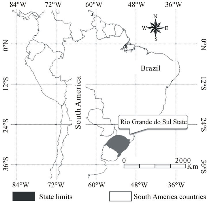
Figure 1. Location of RS in Brazil.
15%), once soybean is a highly mechanized crop and requires relatively smooth land to allow the traffic of farm implements [38];
○ Precipitation data: yearly rainfall data (2000 to 2011) in 30 days accumulated precipitation from 16 meteorological stations, during the period from October to February. These data, from FEPAGRO (Fundação Estadual de Pesquisa Agropecuária—State Foundation for Agriculture and Livestock Research) were used to refine the period of initial sowing and evaluation of total precipitation during crop development.
• Validation data:
○ Annual soybean agricultural statistics, at State and municipality level from [39] for the entire study area. These official statistics were used to compare and evaluate the production results obtained from CM;
○ A second source of information, annual soybean agricultural statistics, at State level from [33] was used for the entire study area. These data were used also to compare and evaluate the results obtained from the present soybean production estimation procedure together with IBGE official statistics data;
○ Crop level data obtained from Technical Report [40] on 2008/2009 crop year were used for spatial validation process. For each one of crop sample points, the crop type and yield were identified.
The input data for the CM are the Enhanced Vegetation Index (EVI). The EVI is part of the MOD13Q1-V005 product, which comprises the best radiometric and geometric pixels selected within a 16-day period. EVI is aindicator of vegetation vigor which is based on canopy reflectance characteristics of vegetation, and was developed to minimize ground influence and atmospheric effects in order to accurately represent vegetated areas by means of satellite measures [41]. EVI data were chosen due to their potential ability to reduce atmospheric and soil background effects [16,42]. The EVI formulation is 2.5(Nir-Red)/(Nir + 6 Red − 7.5 Blue + 1), in which: Nir, Red, and Blue are atmospherically or partially-atmospherically corrected surface reflectance of near infrared, red, and blue bands, respectively [42]. The MODIS images and its products were preprocessed by the National Aeronautics and Space Administration (NASA) and are available at no charge at the [43].
2.3. CM: Methodological Approach
An operational crop yield model should be based on adtations to specific regional agricultural calendars in a knowledge-driven approach, instead of a data-driven approach which is based on data samples for training classification algorithms [18]. The profile of the crop cycle development related to crop vigor is parameterized from EVI data. The methodology developed for soybean yield estimate, in a pixel basis, was named MODIS Productivity Detection Model (MPDM). MPDM is a mathematical approach for soybean yield estimate based on identifying the main PDC acting in the crop development profile of vegetation [1,18] which modulates the EVI from sowing/planting to maximum vegetation development. CM is a coupled model obtained by combining MCDA for area estimate and MPDM for yield. According to CM procedure, soybean EVI profile is expected to have low values during the sowing period and high values at maximum vegetation development. Following the sowing period, a rapid increase of the MODIS/EVI values is observed due to intense plant growth, reaching maximum values in a relative short period [17]. This crop development pattern, as a primary concept, was postulated considering that the complete vegetation development profile is representative of the total agrometerological conditions and management practices acting during development of plants. This approach is based primarily on the following Vegetation Physical Concepts (VPC):
1) A complete crop development profile is representative of crop vegetation vigor;
2) The area calculated between the crop profile graph described as a function of EVI, and above zero, is proportional to the maximum crop production, in order that different crop development conditions sweep out different areas during equal time windows in the same period. So, the calculated area is representative of the maximum crop yield possible to the soybean culture, in the specific crop year, in the studied region;
3) Considering as truth points 1 and 2, crop development in RS reaches its maximum within a fixed window period, from 017 to 049 day-of-year (DOY).
Once the crop profile reaches its maximum, and flattens off, the calculation of maximum EVI value of current crop is obtained by averaging it in the fixed time window (according to item 3 of VPC).
Based on these concepts, the remaining challenge is to understand the main PDC related to factors that do not cause detectable effects on vegetation growth but do constrain the grain production. Reference [27] observed that the flowering period of seasonal agricultural vegetation is more sensitive to temperature than to water stress. In this way, the selected time window covers the flowering period to grain filling and can be calculated by a simple Riemann Integration, and is fundamental to a knowledge-driven approach concept.
Figure 2 shows a trend line with standard deviation markers of crop yield as function of integrated EVI profile of soybean crop from 2000/2001 to 2010/2011. Integrated EVI was obtained from the average of the time window of maximum vegetation development. Three consecutive EVI images from the maximum plant growth were used to obtain integrated EVI which is referred as max EVI window. The resulting max EVI window image
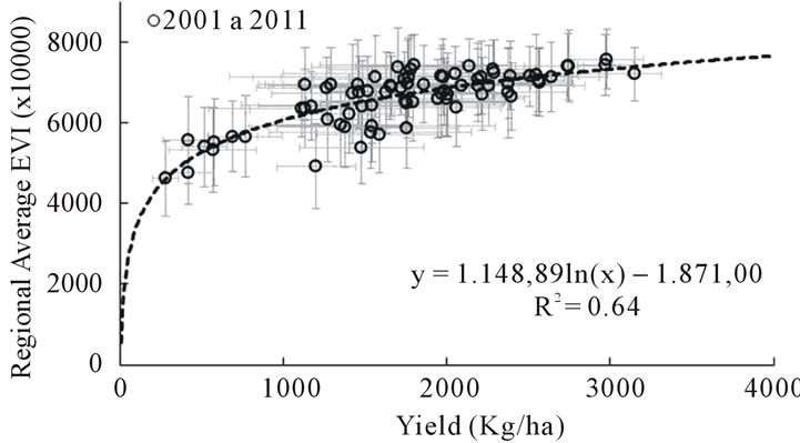
Figure 2. Regional averages of integrated EVI as function of regional averages of soybean yield from 2000/2001 to 2010/ 2011.
is the average from the three consecutive images. Each crop year has eight administrative regions.
Coupling the two processes (MCDA and MPDM) generate results, at a pixel basis that can be described by a single non-linear mathematical function that relates the integrated value to yield. Output values that were obtained by applying this approach are representative of integrating physical conditions of the crop vegetation development through time.
Based on this approach, parameterizations were performed during the development cycle of culture that can be best represented by images of vegetation index [3] using statistical data from official agricultural institutions of Brazil and crop campaign data.
The mathematical relation that links crop vigor profile development to grain production, at the plant level through time, is used to link spatial distribution of EVI at intra-annual basis by means of a simple associative transfer property.
CM estimation is obtained by using a simplified approach which is based solely on EVI images as input parameter. Soybean yield estimation can be provided right after a set of EVI images become available, which normally occurs in early February. CM works on calculating the soybean yield, in a per pixel basis, by means the mathematical rule which relates the vegetation vigor from EVI values to yield in the entire max EVI window. However, only the EVI values associated to soybean crop area selected from MCDA will be considered. In this way, pixels which fall out from soybean crop areas are tagged as zero yield.
A delay of about 20 days is expected in order to acquire the MOD13Q1 product; and therefore, soybean estimation should be released no later than early March.
It is important to emphasize that the parameters defined in CM for crop production estimate are constant as a fixed criteria of CM equation, during the period we studied (eleven crop years between 2000/2001 and 2010/ 2011) independently of the soybean crop development or multi-year dynamics in RS State. When any further adjustment of parameters is needed, in order to plot a better fitting of the seasonal crop yield during the calibration procedure, a new test cycle is started for all crops. It means that by considering the main PDC as representative of soybean crop development profile, revealing the correlation between crop vigor and total municipal production, it is expected that a set of constants parameters will be able to be adjusted as fixed criteria. Therefore, once identified the mathematical parameters related to the PDC, no post-adjustment was allowed.
3. Results
Soybean production in RS State was compared to official estimates from IBGE and CONAB at State and municipality level from 2000/2001 to2010/2011. Figures 3 and 4 show the high variability in production and yield due to seasonal agrometeorological conditions in RS. Interpolated maps were obtained from averages in the period from 2000/2001 to 2010/2011, since the most recent municipal information for 2011/2012 had not yet been released by IBGE. Table 1 presents the crop level estimates using local level data.
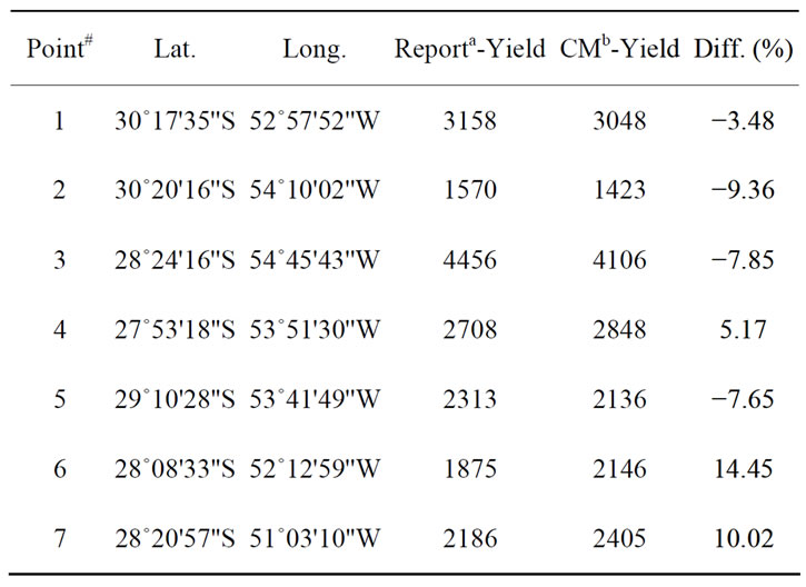
Table 1. Location of the sample points obtained in 2008/ 2009 crop year from Dotto and Rosinha (2009) [40].
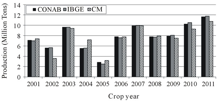
Figure 3. Comparison of total production estimates between IBGE and CM for each crop year, from 2000/2001 to 2010/ 2011.
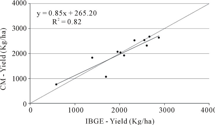
Figure 4. Scatterplot showing the trend line of soybean yield between IBGE and CM estimates, for each crop year, from 2000/2001 to 2010/2011.
3.1. State Level Analysis
Linear least squares regression analysis was done for State level soybean yield estimates obtained from IBGE and CM for 2000/2001 to 2010/2011 crop years. Figure 3 compares the total soybean production in the State from IBGE and CM.
Production estimates with CM is obtained for each pixel multiplying yield by pixel area (pixel of 250 m is 6.25 ha). CM exhibits trend to underestimate yield when comparing to IBGE. Results obtained by Melo et al. (2008) [10], analyzing the performance modeling using images of low spatial resolution (9 km), between 1975 and 2000, obtained a correlation coefficient (Pearson correlation) R = 0.96, when they considered fitting to all points. Reference [13] evaluated several regions of Brazil. In RS, they found a correlation coefficient of R = 0.26. In Figure 4, it is observed the most pronounced point positioned below the linear least squares regression function. Where IBGE declares a yield average of 1708 Kg/ha, CM yield estimate is 1068 Kg/ha, which represents a difference of −37.1% in the crop year 2001/2002.
Analysis of precipitation distribution in 2001/2002 shows a lower than normal trend from southwestern region of the State towards the north region, where is the most intensive soybean crop fields.
Figure 5 shows the percent deviation of cumulative precipitation in 2001/2002, based in the climatological normal (1971 to 2000) obtained with analysis of interpolated maps.
By comparing these maps, a large difference is revealed not only in the distribution of precipitation, but also in the total amount all over the State. This result leads to an interpretation of overestimated IBGE production in 2001/2002 because the amount of precipitation that occurred in summer crop of 2001/2002 was not suitable to the resulting yield from IBGE.
Figure 6 shows the yield deviation of CM from IBGE in summer crop of 2001/2002.
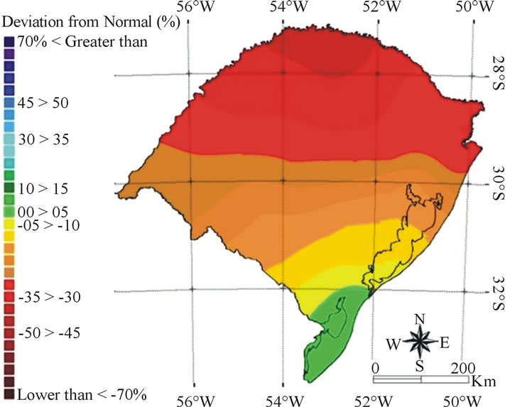
Figure 5. Percent deviationof cumulative precipitation in thecrop year 2001/2002, starting from normal climatological conditions (1971 to 1990).
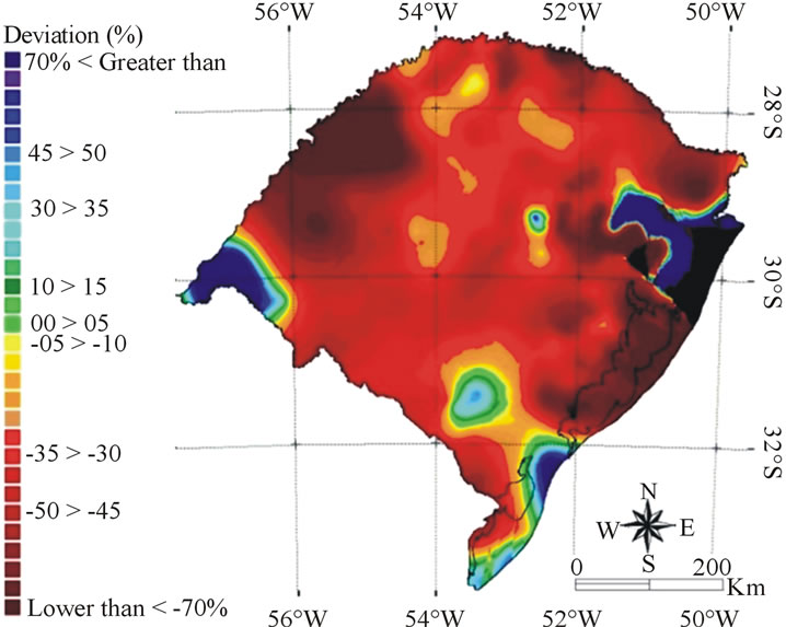
Figure 6. Percent deviation of soybean yield with CM in the crop year 2001/2002, starting from municipality data of IBGE.
The deviation trend do not shows the expected increasing in the yield deviation towards the north, which is related to deviations of precipitation greater than 30%, as shown in Figure 5. Also, it is important to note in Figure 6 the great dark-red area in the north-west region in RS State. This region showed the most pronounced negative yield differences where CM estimates are more than 50% below IBGE in 2001/2002. Usually, this is the most affected area by droughts in RS, which results in a soybean yield lower than average for longer periods. The dark-blue regions are related to small farms with high soybean yield. As a result, interpolated maps of yield estimates from CM, compare centroids which does not has any soybean production to another ones which has above average yields.
In Figure 4, the coefficient of determination is R2 = 0.82. Considering previous observations from IBGE, the soybean yield distribution in 2001/2002, it is an outlier, andso, it has to be extracted from validation crop years. The new coefficient of determination found is R2 = 0.91 indicating that CM trend is in good agreement with total production of State level estimates.
3.2. Municipality Level Estimates
Figure 7 presents CM map of soybean yield in 2010/ 2011 crop year. CM map is able to generate data at municipal scale or intra-municipal scale due to its 250 m full resolution. At municipality level, scatterplot in Figure 8 shows the grouping of points along the symmetry line in the inter-comparison between total production obtained from CM and obtained from the IBGE, in all crop years from 2000/2001 to 2010/2011.
There is a trend of CM to overestimate production in comparison to IBGE which is not observed in the State level analysis of yield (Figure 4). The same is observed at municipality level. At yearly based analysis, coefficients of determination (R2) ranged from 0.90 to 0.95 indicating
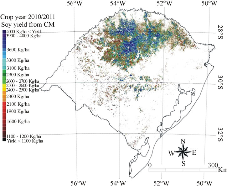
Figure 7. Soybean yield in 2010/2011 crop year from CM.
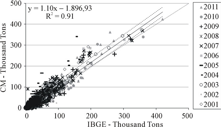
Figure 8. Scatterplot comparing municipality estimates of production in RS, between IBGE and CM, from 2000/2001 to 2010/2011.
good agreement between estimates. The majority of slope coefficients values ranged around 1.10, which indicates that CM overestimated the soybean production in relation to IBGE for municipalities with highest production.
In Figure 8, the four points placed above 350,000 tons are representative of soybean production in the municipality of Tupanciretã, which already in 2003 was the major producer in RS with more than 355,000 tons [39]. The RMSD is 10,840 tons for all aggregated data of crop years. Considering a double RMSD from trend line, 95% of occurrences are in between dashed lines indicating that CM estimates are consistent.
3.3. Local Level Analysis
The local level analysis was performed by using yield estimates in the 2008/2009 crop year from the Crop Production Report, by [40]. Local level comparison must be evaluated carefully due to the nature of different scales measures in this comparison. It is expected a high spatial variability of plant level analysis which may not be representative of the large scale crop yield, and so, when comparing moderate resolution (250 m) and crop level data (plant yield). Results obtained from the CM approach shows that the CM estimations adhere to spatial variability of yield obtained from the seven sampled points in different locations with coordinates presented in Table 1. The obtained coefficient of determination (R2) is 0.95 and the slope coefficient is 0.86.
4. Conclusions
The CM approach is based on a consistent and objective methodology for regional estimation of soybean production using MODIS/EVI imagery.
Implementing operational crop yield forecasts in advance to crop harvest remains a challenge at regional scale, since it implies to model different scale levels. Also, it implies to take into account a large set of local level data, which is not commonly available or easily provided.
By using pre-defined parameters, CM approach demonstrated to be able to provide complementary information of yield and production forecasts in advance to crop harvest, being less subjected to complex time-expensive analytical methodologies and image interpretation.
Further analysis and developments for CM must be undertaken in Mato Grosso State, Brazil, where far different ecoregions characteristics from Rio Grande do Sul State prevail. Additionally, local level data are subject to different impacts of physically-driven components as crop variety and local agrometeorology.
5. Acknowledgements
The authors are thankful to Fundação Estadual de Pesquisa Agropecuária do Rio Grande do Sul (FEPAGRO). Special thanks are due to Conselho Nacional de Desenvolvimento Científico e Tecnológico (CNPq).
REFERENCES
- A. Gusso, “Integração de imagens NOAA/AVHRR: Rede de Cooperação Para Monitoramento Nacional da Safra de Soja,” Revista Ceres, Vol. 60, No. 2, 2013, pp. 194-204. http://dx.doi.org/10.1590/S0034-737X2013000200007
- D. C. Figueiredo, “Projeto GeoSafras: Aperfeiçoamento do Sistema de Previsão de Safras da Conab,” Revista de Política Agrícola, Vol. 14, 2005, pp. 110-120.
- A. Gusso, A. R. Formaggio, R. Rizzi, M. Adami and B. T. F. Rudorff. “Soybean Crop Area Estimation by MODIS/ EVI Data,” Pesquisa Agropecuária Brasileira, Vol. 47, No. 3, 2012, pp. 425-435. http://dx.doi.org/10.1590/S0100-204X2012000300015
- J. A. Johann, J. V. Rocha, D. G. Duft and R. A. C. Lamparelli, “Estimativa de Áreas com Culturas de Verão no Paraná, por Meio de Imagens Multitemporais EVI/Modis,” Pesquisa Agropecuária Brasileira, Vol. 47, No. 9, 2012, pp. 1295-1306. http://dx.doi.org/10.1590/S0100-204X2012000900015
- R. Rizzi and B. T. F. Rudorff, “Imagens do Sensor MODIS Associadas a um Modelo Agronômicopara Estimar a Produtividade de Soja,” Pesquisa Agropecuária Brasileira, Vol. 42, No. 1, 2007, pp. 73-80. http://dx.doi.org/10.1590/S0100-204X2007000100010
- E. D. Assad, F. R. Marin, S. R. Evangelista, F. G. Pilau, J. R. B. Farias, H. S. Pintoand and J. Zullo, “Sistema de Previsão da Safra de Soja para o Brasil,” Pesquisa Agropecuária Brasileira, Vol. 42, No. 5, 2007, pp. 615-625. http://dx.doi.org/10.1590/S0100-204X2007000500002
- E. E. Sano, L. G. Ferreira, G. P. Asner and E. T. Steinke, “Spatial and Temporal Probabilities of Obtaining CloudFree Landsat Images over the Brazilian Tropical Savanna,” International Journal of Remote Sensing, Vol. 28, No. 12, 2007, pp. 2739-2752. http://dx.doi.org/10.1080/01431160600981517
- L. M. Sugawara, B. F. T. Rudorff and M. Adami, “Viabilidade de Uso de Imagens do Landsat em Mapeamento de área Cultivada com Soja no Estado do Paraná,” Pesquisa Agropecuária Brasileira, Vol. 43, No. 12, 2008, pp. 1763-1768. http://dx.doi.org/10.1590/S0100-204X2008001200019
- J. C. D. M. Esquerdo, J. Zullo and J. F. G. Antunes, “Use of NDVI/AVHRR Time-Series Profiles for Soybean Crop Monitoring in Brazil,” International Journal of Remote Sensing, Vol. 32, No. 13, 2011, pp. 3711-3727. http://dx.doi.org/10.1080/01431161003764112
- R. W. De Melo, D. C. Fontana, M. A. Berlato and J. R. Ducati, “An Agrometeorologica-Spectral Model to Estimate Soybean Yield, Applied to Southern Brazil,” International Journal of Remote Sensing, Vol. 29, No. 14, 2008, pp. 4013-4028. http://dx.doi.org/10.1080/01431160701881905
- D. A. Sims, A. F. Rahman, V. D. Cordova, B. Z. El-Masri, D. D. Baldocchi, P. V. Bolstad, L. B. Flanagan, A. H. Goldstein, D. Y. Hollinger, L. Misson, R. K. Monson, W. C. Oechel, H. P. Schmid, S. C. Wofsy and L. Xu, “On the Use of MODIS EVI to Assess Gross Primary Productivity of North American Ecosystems,” Journal of Geophysical Research, Vol. 111, No. G4, 2006, pp. 1-16. http://dx.doi.org/10.1029/2006JG000162
- P. C. Doraiswamy, T. R. Sinclair, S. Hollinger, B. Akhmedov, A. Stern and J. Prueger, “Application of MODIS Derived Parameters for Regional Crop Yield Assessment,” Remote Sensing of Environment, Vol. 97, No. 2, 2005, pp. 192-202. http://dx.doi.org/10.1016/j.rse.2005.03.015
- W. T. Liu and F. Kogan, “Monitoring Brazilian Soybean Production Using NOAA/AVHRR Based Vegetation Indices,” International Journal of Remote Sensing, Vol. 23, No. 3, 2002, pp. 1161-1180.
- D. C. Fontana, E. Weber, J. R. Ducati, M. A. Berlato, L. A. Guasselli and A. Gusso, “Monitoramento da Cultura da Soja no Centro-Sul do Brasil Durante La Niña de 1998/2000,” Revista Brasileira de Agrometeorologia, Vol. 10, No. 6, 2002, pp. 343-351. http://dx.doi.org/10.1080/01431160110076126
- D. B. Lobell and G. P. Asner, “Cropland Distributions from Temporal Unmixing of MODIS Data,” Remote Sensing of Environment, Vol. 93, No. 3, 2004, pp. 412-422. http://dx.doi.org/10.1016/j.rse.2004.08.002
- C. O. Justice, J. R. G. Townshend, E. F. Vermote, E. Masuoka, R. E. Wolfe, N. Saleous, D. P. Roy and J. T. Morisette, “An Overview of MODIS Land Data Processing and Product Status,” Remote Sensing of Environment, Vol. 83, No. 1-2, 2002, pp. 3-15. http://dx.doi.org/10.1016/S0034-4257(02)00084-6
- B. D. Wardlow, S. L. Egbert and J. H. Kastens, “Analysis of Time-Series MODIS 250m Vegetation Index Data for Crop Classification in the US Central Great Plains,” Remote Sensing of Environment, Vol. 108, No. 3, 2007, pp. 290-310. http://dx.doi.org/10.1016/j.rse.2006.11.021
- A. Gusso and J. R. Ducati, “Algorithm for Soybean Classification Using Medium Resolution Satellite Images,” Remote Sensing, Vol. 4, No. 10, 2012, pp. 3127-3142. http://dx.doi.org/10.3390/rs4103127
- D. Arvor, M. Jonathan, M. S. P. Meirelles, V. Dubreuil and L. Durieux, “Classification of MODIS EVI Time Series for Crop Mapping in the State of Mato Grosso, Brazil,” International Journal of Remote Sensing, Vol. 29, No. 22, 2011, pp. 1-25.
- R. Rizzi and B. F. T. Rudorff, “Estimativa da Área de Plantada com Soja no Rio Grande do Sul por Meio de Imagens Landsat,” Revista Brasileira de Cartografia, Vol. 57, No. 3, 2005, pp. 226-234.
- R. D. V. Epiphanio, A. R. Formaggio, B. T. F. Rudorff, E. E. Maeda and A. J. B. Luiz, “Estimating Soybean Crop Areas Using Spectral-Temporal Surfaces Derived from MODIS Images in Mato Grosso, Brazil,” Pesquisa Agropecuária Brasileira, Vol. 45, No. 1, 2010, pp. 72-80. http://dx.doi.org/10.1590/S0100-204X2010000100010
- D. C. Morton, R. S. DeFries, Y. E. Shimabukuro, L. O. Anderson, E. Arai, F. D.-B. Espirito-Santo, R. Freitas and J. Morissete, “Cropland Expansion Changes Deforestation Dynamics in the Southern Brazilian Amazon,” Proceedings of the National Academy of Sciences, Vol. 103, No. 39, 2006, pp. 14637-14641.
- M. N. Macedo, R. S. DeFries, D. C. Morton, C. M. Stickler, G. L. Glaford and Y. E. Shimabukuro, “Decoupling of Deforestation and Soy Production in the Southern Amazon during the late 2000s,” Proceedings of the National Academy of Sciences, Vol. 109, No. 4, 2006, pp. 1341-1346. http://dx.doi.org/10.1073/pnas.1111374109
- K. Pittman, M. C. Hansen, I. Becker-Reshef, P. V. Potapov and C. O. Justice, “Estimating Global Cropland Extent with Multi-Year MODIS Data,” Remote Sensing, Vol. 2, No. 7, 2010, pp. 1844-1863. http://dx.doi.org/10.3390/rs2071844
- D. B. Ferreira,“Análise da Variabilidade Climática e Suas Consequencias Para a Produtividade da Soja na Região sul do Brasil,” Ph.D. Thesis, INPE, São José dos Campos, 2010.
- W. Schlenker and M. Roberts, “Nonlinear Temperature Effects Indicate Severe Damages to US Crop Yields under Climate Change,” Proceedings of the National Academy of Sciences. Vol. 106, No. 37, 2009, pp. 15594- 15598. http://dx.doi.org/10.1073/pnas.0906865106
- F. N. Kogan, “Operational Space Technology for Global Vegetation Assessment,” Bulletin of American Meteorological Society, Vol. 82, No. 9, 2001, pp. 1949-1964. http://dx.doi.org/10.1175/1520-0477(2001)082<1949:OSTFGV>2.3.CO;2
- C. O. Justice, G. Dugdale, J. R. G. Townshend, A. S. Narracott and M. Kumar, “Synergism between NOAAAVHRR and Meteosat Data for Studying Vegetation Development in Semi-Arid West Africa,” International Journal of Remote Sensing, Vol. 12, No. 6, 1991, pp. 1349- 1368. http://dx.doi.org/10.1080/01431169108929730
- D. A. Sims, A. F. Rahman, V. D. Cordova, B. Z. El-Masri, D. D. Baldocchi, P. V. Bolstad, L. B. Flanagan, A. H. Goldstein, D. Y. Hollinger, L. Misson, R. K. Monson, W. C. Oechel, H. P. Schmid, S. C. Wofsy and L. Xu, “A New Model of Gross Primary Productivity for North American Ecosystems Based Solely on the Enhanced Vegetation Index and Land Surface Temperature from MODIS,” Remote Sensing of Environment, Vol. 112, No. 4, 2008, pp. 1633-1646. http://dx.doi.org/10.1016/j.rse.2007.08.004
- F. N. Kogan, “World Droughts in the Millennium from AVHRR-Based Vegetation Health Indices,” Eos, Transactions, American Geophysical Union, Vol. 83, No. 48, 2002, pp. 557-564. http://dx.doi.org/10.1029/2002EO000382
- A. O. Cardoso, A. M. H. de Avila, H. S. Pinto and E. D. Assad, “Use of Climate Forecasts to Soybean Yield Estimates,” In: H. El-Shemy, Ed., Soybean Physiology and Biochemistry, InTech, 2011, p. 489. http://www.intechopen.com/books/soybean-physiology-and-biochemistry/
- E. Mercante, R. A. C. Lamparelli, M. A. Uribe-Opazo and J. V. Rocha, “Modelos de Regressão Lineares Para Estimativa de Produtividade da Soja no Oeste do Paraná, Utilizando Dados Espectrais,” Engenharia Agrícola, Vol. 30, No. 3, 2010, pp. 504-517. http://www.scielo.br/scielo.php?pid=S0100-69162010000300014&script=sci_arttext
- CONAB, “Companhia Nacional de Abastecimento. Historical Series,” 2011. http://www.conab.gov.br/conteudos.php?a=1252&t=2&Pagina_objcmsconteudos=3#A_objcmsconteudos
- K. R. Saraiva and F. Souza, “Estatísticas Sobre Irrigação nas Regiões Sul e Sudeste do Brasil Segundo o Censo Agropecuário 2005-2006,” Revista Irriga, Vol. 16, No. 2, 2012, pp. 168-176.
- J. Paulino, M. V. Folegatti, C. A. Zolin, R. M. SánchezRomán and J. V. J. Unesp, “Situação da Agricultura Irrigada no Brasil de Acordo com o Censo Agropecuário 2006,” Irriga, Vol. 16, No. 3, 2011, pp. 163-176.
- G. R. da Cunha, N. A. Barni, J. C. Haas, J. R. T. Maluf, R. Matzenauer, A. Pasinato, M. B. M. Pimentel and J. L. F. Pires, “Zoneamento Agrícola e Época de Semeadura Para Soja No Rio Grande do Sul,” Revista Brasileira de Agrometeorologia, Vol. 9, No. 3, 2001, pp. 446-459.
- B. M. Rabus and A. R. R. Eineder, “The Shuttle Radar Topography Mission—A New Class of Digital Elevation Models Acquired by Spaceborneradar,” Photogrammetric Engineering & Remote Sensing, Vol. 57, No. 4, 2003, pp. 241-262. http://dx.doi.org/10.1016/S0924-2716(02)00124-7
- E. Jasinski, D. Morton, R. DeFries, Y. Shimabukuro, L. Anderson and M. Hansen, “Physical Landscape Correlates of the Expansion of Mechanized Agriculture in Mato Grosso, Brazil,” Earth Interactions, Vol. 9, No. 16, 2005, pp. 1-18. http://dx.doi.org/10.1175/EI143.1
- Instituto Brasileiro de Geografia e Estatística (IBGE), “Produção Agrícola Municipal—Automatic Data Recovery System—SIDRA,” 2011. www.sidra.ibge.gov.br
- S. R. Dottoand and R. C. Rosinha, “Desempenho de Cultivares de Soja Indicadas Para o RS-Relatório de Produtividade, Resultados 2008/2009,” Fundação Pró-Sementes/Sistema FARSUL, 2009.
- P. M. Brando, S. J. Goetz, A. Baccini, D. C. Nepstad, P. S. A. Beck and M. C. Christman, “Seasonal and Interanual Variability of Climate and Vegetation Indicies across the Amazon,” Proceedings of the National Academy of Sciences of the United States of America, Vol. 107, No. 33, pp. 14685-14690. http://dx.doi.org/10.1073/pnas.0908741107
- A. Huete, K. Didan, T. Miura, E. P. Rodriguez, X. Gao and L. G. Ferreira, “Overview of the Radiometric and Biophysical Performance of the MODIS Vegetation Indices,” Remote Sensing of Environment, Vol. 83, No. 1-2, 2002, pp. 195-213. http://dx.doi.org/10.1016/S0034-4257(02)00096-2
- National Aeronautics and Space Administration (NASA), “Warehouse Inventory Search Tool,” 2009.
NOTES
*Simplified model for soybean yield based solely on MODIS/EVI data.
#Corresponding author.