International Journal of Geosciences
Vol.4 No.4(2013), Article ID:33344,9 pages DOI:10.4236/ijg.2013.44061
Modeling of Atmospheric Gravity Effects for High-Precision Observations
Institut für Erdmessung, Leibniz Universität Hannover, Hannover, Germany
Email: gitlein@ife.uni-hannover.de
Copyright © 2013 Olga Gitlein et al. This is an open access article distributed under the Creative Commons Attribution License, which permits unrestricted use, distribution, and reproduction in any medium, provided the original work is properly cited.
Received April 15, 2013; revised May 16, 2013; accepted June 13, 2013
Keywords: Atmospheric Reduction; Green’s Functions; ECMWF; Absolute Gravimetry; Superconducting Gravimeter
ABSTRACT
Temporal variations of atmospheric density distribution induce changes in the gravitational air mass attraction at a specific observation site. Additionally, the load of the atmospheric masses deforms the Earth’s crust and the sea surface. Variations in the local gravity acceleration and atmospheric pressure are known to be corrected with an admittance of about 3 nm/s2 per hPa as a standard factor, which is in accordance with the IAG Resolution No. 9, 1983. A more accurate admittance factor for a gravity station is varying with time and depends on the total global mass distribution within the atmosphere. The Institut für Erdmessung (IfE) performed absolute gravity observations in the Fennoscandian land uplift area nearly every year from 2003 to 2008. The objective is to ensure a reduction with 3 nm/s2 accuracy. Therefore, atmospheric gravity changes are modeled using globally distributed ECMWF data. The attraction effect from the local zone around the gravity station is calculated with ECMWF 3D weather data describing different pressure levels up to a height of 50 km. To model the regional and global attraction, and all deformation components the Green’s functions method and surface ECMWF 2D weather data are used. For the annually performed absolute gravimetry determinations, this approach improved the reductions by 8 nm/s2 (−19 nm/s2 to +4 nm/s2). The gravity modeling was verified using superconducting gravimeter data at station Membach in Belgium improving the residuals by about 15%.
1. Introduction
Since the end of last glacial period the Fennoscandian shield rises in the uplift centre about 1 cm per year resp. −16 nm/s2 per cm, cf. [1]. The lithosphere responses to its original position due to deloading of ice. This uplift is observed by geometric and gravimetric methods [1-4]. A joint project for gravimetric surveys of the land uplift in Fennoscandia was established in 2003 within a multinational cooperation. Annual measurements with the absolute gravimeter were performed in Fennoscandia from 2003 to 2008 by the Institut für Erdmessung (IfE) from the Leibniz Universität Hannover, Germany. Figure 1 shows the stations occupied by IfE with FG5-220; in total 31 different stations mostly co-located with permanent GPS. In [5] a summary of all gravity measurements and the results of the IfE surveys are given.
The gravimeter measures effects of different sources and is an “integral” sensor. The observations have to be reduced by time variable gravity changes due to solid Earth and ocean tides, polar motion, and atmospheric variations. An uncertainty of ±3 nm/s2 or even better is striven for each reduction to ensure the high accuracy of FG5 absolute gravimeter results.
Atmospheric mass redistributions cause temporal variations of density and thus of gravity of several 100 nm/s2. The local gravity is affected directly by the Newtonian attraction of the globally distributed air masses as well as indirectly by the height shifts of the Earth’s surface and mass redistributions within the Earth’s crust.
Usually, the atmospheric effect is considered with a global average regression coefficient of −3 nm/s2 per hPa applying the local air pressure measurements at the gravimetry station, cf. IAG Resolution No. 9, 1983. The air pressure measurement at ground level shows the density changes as an integral effect of the atmospheric vertical column. This simplified reduction approach does not consider the real mass movements within the global atmosphere thus unmodeled gravity effects of some 10 nm/s2 can remain. Therefore, in this paper the gravity effects (attraction and deformation), cf. [6], are modeled based on globally distributed 2D and 3D weather data from ECMWF (European Centre for Medium-Range Weather Forecasts). Previous studies apply reductions to
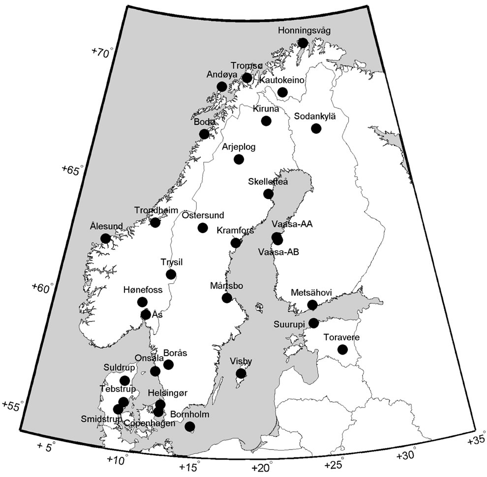
Figure 1. Absolute gravity stations occupied with FG5-220 from 2003 to 2008 by Institut für Erdmessung, Leibniz Universität Hannover; in total 31 stations.
continuous records with superconducting gravimeters, VLBI, GPS, and SLR techniques, cf. [7-18].
2. Modeling of Atmospheric Gravity Effects
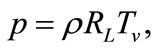
Global 2D and 3D from ECMWF are used, which are logged every 6 hours on a 1.125˚ × 1.125˚ grid for 2D data and 0.75˚ × 0.75˚ grid in 21 pressure levels (1000 to 1 hPa) for 3D data. The data contain meteorological parameters as barometric pressure p, geopotential V, temperature T and relative humidity r. They allow to model the Newtonian attraction of air volumes with sizes corresponding to the given data grid and pressure levels. To calculate the required air density, the gas law gives the relationship between air pressure p, density p, and temperature T (here virtual temperature ) as
) as
 (1)
(1)
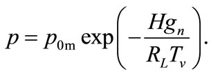
where by  is the gas constant for dry air. The distribution of air masses within a column follows approximately a mathematical approach on the basis of atmospheric surface data like air pressure and temperature. Air pressure, temperature, density, and height H are interdependent and follow the known “barometric height formula”, which shows the exponential decrease of air pressure with height [19].
  is the air pressure at sea level with height 0 m and
  m/s2 is the mean gravity at the geoid:
 (2)
(2)
2.1. Gravity Using Green’s Functions and 2D Data
The direct gravitational effect of air mass changes and the effect of pressure loading on the Earth’s surface can be represented mathematically. A transition from volume to surface integrals can be achieved with Green’s functions. [20,21] introduced Green’s functions for a point mass load to calculate the elastic deformation effects of the Earth’s crust due to ocean tides. This thin layer of ocean variation can be modeled as a point mass grid. With respect to Earth’s atmosphere the masses are distributed vertically in a column and the Newtonian attraction must be considered for a 3-dimensional volume. Due to the transition from volume to surface integrals, the Green’s functions only depend on 2D surface data as defined at sea level. Calculation algorithms and results of atmospheric Green’s functions can be found in, e.g., [10, 12,22,23]. In this paper the Green’s functions of [22] are applied for the gravity modeling.
The total gravity effect of an air column with the area A at base (in steradian) and the spherical distance  between the column base and the gravimeter is given by
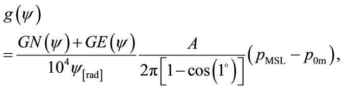 (3)
(3)
in [nm/s2], cf. [6,10,22]. The effect  depends on air pressure
  at mean sea level, and on Green’s functions for Newtonian attraction
  and elastic deformation
 . The difference between the real surface temperature and the reference temperature (15˚C) is considered as a correction term in
 . In the ocean area air mass variations do not deform the ocean bottom but change water levels [8,24-27]. This hypothesis of the inverted barometer effect is also applied in calculations of loading effects for records with VLBI, SLR, GPS, and superconducting gravimeters [8,13-16,28-31]. To meet the IAG Resolution No. 9 of 1983 for absolute gravimetry, cf. [32], the real atmospheric variations are referred to the standard atmosphere. Therefore, the reference air pressure at sea level
  hPa is considered for all air pressure data
  at mean sea level in Equation (3).
Green’s functions vary with spherical distance . The globally distributed ECMWF weather data are subdivided into three grid zones around the computation point (gravity station) and interpolated with different grid resolutions:
• local zone with  and 0.005˚ × 0.005˚• regional zone with
  and 0.1˚ × 0.1˚, and
• global zone with  and 1.125˚ × 1.125˚.
Total gravity effect for each zone is obtained by summing up all small effects  of each grid point with the distance
  to computation point, Equation (3).
2.2. Attraction from Local Zone Using 3D Data
The direct attraction effect of air mass changes from the local zone contributes more than 80% to the total gravity effect. Air density changes along the vertical within the air column cause measurable gravity signal although the air pressure at surface (2D) remains constant. Calculated Green’s functions of [22] are based on a model atmosphere. The considered model is a mean situation over all seasons and does not show the actual situation in higher air layers. Consequently, the mass redistribution within the atmosphere can not be modeled exactly with only Green’s functions and surface data (2D). Therefore, the gravitational effect from the local zone is calculated directly by Newton’s law of gravity using 3D data from ECMWF, cf. [6]. Gravity variations caused by vertical air mass displacement can reach several 10 nm/s2, [6,17, 33,34]. This contribution is not considered using the classical reduction method with station air pressure recordings.
[10,35-39] developed methods to calculate the attraction effect of surrounding masses, which are presented in prisms. This procedure is applied for the investigations in this paper. The atmospheric attraction  of a small mass element Q with its volume
  is calculated in a cartesian coordinate system with origin in the computation point (gravity station)
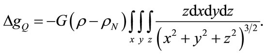 (4)
(4)
The density ρ is determined from pressure, temperature, and humidity given at each level of the ECMWF 3D data, [40,19].  is the density of the US standard atmosphere 1976, which is in accordance with [32] for reductions of absolute gravity. From geopotential V, given at each pressure level, the geometric height z is obtained. Summing up the attraction effects of all small mass volumes
  of Equation (4) yields in the total effect.
3. Verification of Modeling with Superconducting Gravimeter Data
Since 1995 the superconducting gravimeter GWR-C021 (SCG, cf. [41]) is operated continuously at the station Membach in Belgium. Relative gravity changes with a precision of 1 nm/s2 are recorded. Michel Van Camp from the Royal Observatory of Belgium (ROB) kindly provided gravity observations from August 2004 to October 2006. These data are reduced from local and regional hydrological gravity changes [42,43]; they are used to assess the elaborate atmospheric gravity modeling described in Section 2.
3.1. Attraction and Deformation from Different Zones
Based on the calculation algorithm in Section 2.1, attraction and deformation gravity effects are calculated for the station Membach from 01.01.2003 to 31.12.2006. The contributions from the local, regional, global zone, and the air pressure variation are shown on left in Figure 2. The correlation coefficients k between each gravity contribution and station air pressure variation (Figure 2(h)) are given. On the right hand side of Figure 2 the corresponding Fourier amplitude spectra are shown. Table 1 presents the statistics of the results divided into attraction (A) and elastic deformation (E) parts. During the four years the local air pressure varies between −32 and +28 hPa with an RMS of 9 hPa. Hence, atmospheric mass redistributions cause gravity effects with a mean variation of 30 nm/s2 and extrema of −85 nm/s2 and 93 nm/s2. In the following, Table 1 and Figure 2 are discussed with respect to the different zones.
 (a)
(a)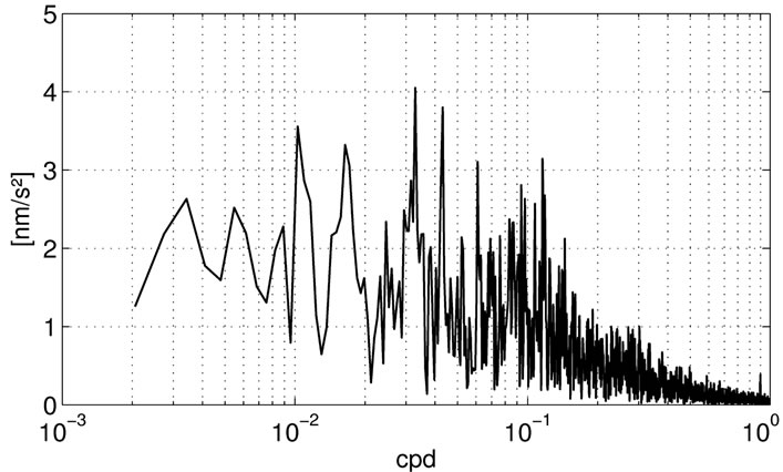 (b)
(b)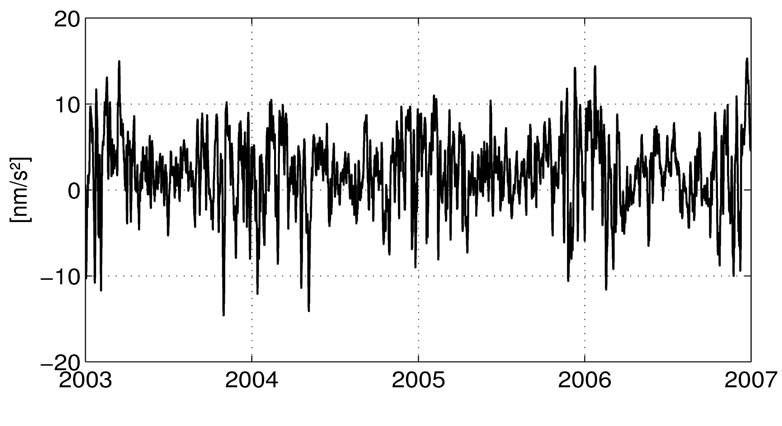 (c)
(c)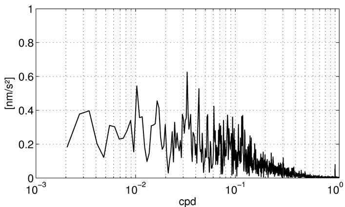 (d)
(d)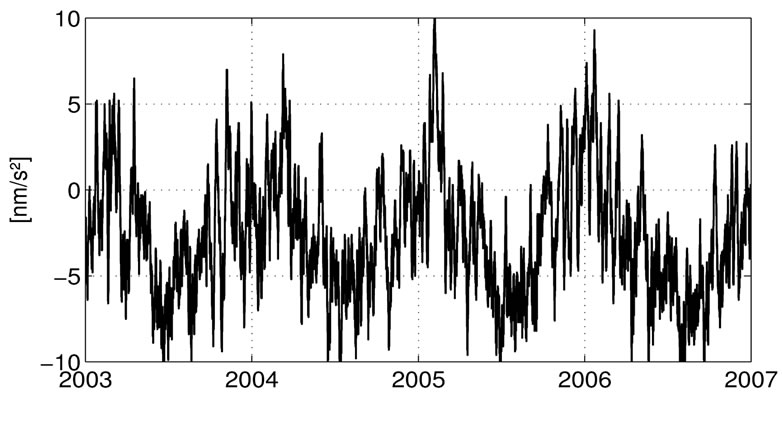 (e)
(e)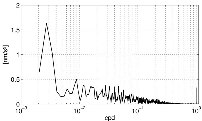 (f)
(f)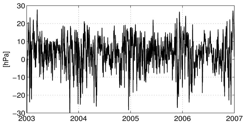 (g)
(g)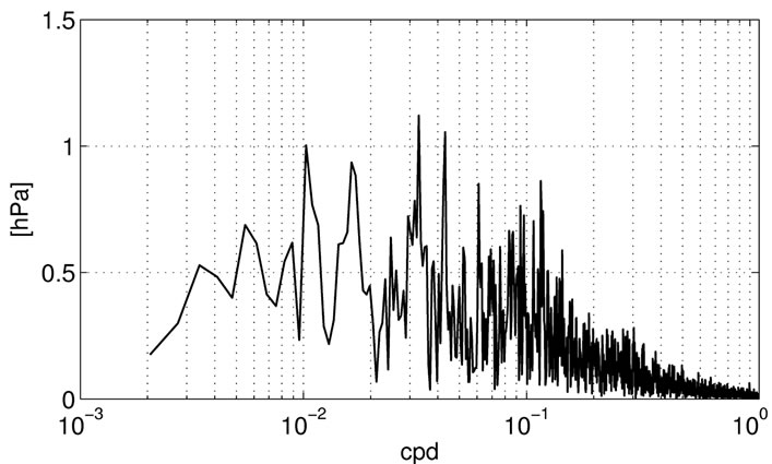 (h)
(h)
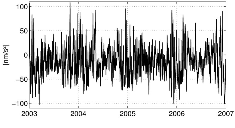
Figure 2. Left: Atmospheric gravity effects from the local, regional, and global zone calculated for the SCG station Membach from atmospheric 2D data between 01.01.2003 and 31.12.2006, and the variation of the station air pressure to normal air pressure. Right: Corresponding Fourier amplitude spectra (cpd: cycles per day). (a) Local effect; correlation k = −0.996; (b) Amplitude spectrum of local effect; (c) Regional effect; correlation k = 0.956; (d) Amplitude spectrum of regional effect; (e) Global effect; correlation k = 0.294; (f) Amplitude spectrum of global effect; (g) Variation of station air pressure; (h) Amplitude spectrum of pressure.
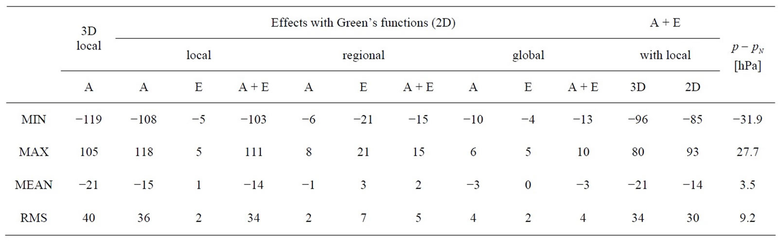
Table 1. Contributions of atmospheric gravity effects in [nm/s2] for Membach from the local, regional, and global zones (A: attraction, E: elastic deformation effect). Effects from the local zone calculated with 2D and 3D data. The station air pressure p obtained from atmospheric 2D data with respect to normal air pressure pn.
• Local zone The effect exceeds with 34 nm/s2 (RMS) the contributions from regional and global zones. Together these two zones contribute about 10% to the total effect of 30 nm/s2. The local attraction dominates significantly with an RMS of 36 nm/s2 compared to local deformation with 2 nm/s2. This effect is negatively correlated with the station air pressure variation. The amplitude spectra of gravity and air pressure are very similar. In spectrum of Figure 2(b) the largest amplitudes are found for periods 97, 60.8, 30.4 and 23 days (0.010, 0.016, 0.033 and 0.043 cpd). The amplitudes decrease continuously in higher frequency ranges above 0.2 cpd. A peak appears at the daily frequency (1 cpd).
• Regional zone The deformation effect dominates with 7 nm/s2 (RMS) compared to attraction with 2 nm/s2. The total contribution varies between −15 and +15 nm/s2 with an RMS of 5 nm/s2. Similar to the local zone, the station air pressure correlates strongly with the gravity, but positively. The amplitude spectra of local and regional gravity effects are similar, but the amplitudes for the regional zone are approximately one order of magnitude smaller. The maximum is found at frequency 0.033 cpd (30.04 days) and is by factor 7 smaller compared to the spectrum of local contribution.
• Global zone These gravity effects vary between −13 and +10 nm/s2 with an RMS of 4 nm/s2. The global effect does not correlate with the local air pressure (compare Figures 2(f) and (h)). Thus, this gravity signal is not considered by the classical air pressure reduction. For high-precision gravimetry applications this gravity contributions should not be neglected. In the spectrum the annual cycle (cpd = 0.0027397) dominates with an amplitude of more than 1.6 nm/s2. A clear peak at daily frequency is found.
3.2. Seasonal Variation of Attraction from Local Zone
Atmospheric attraction gravity effects from the local zone are calculated for the SCG station in Membach using 3D data. Figure 3 shows the difference between 3D and 2D data calculation and the corresponding amplitude spectrum. The 3D modeling shows larger signals in the summer periods. The gravitational center in a vertical column moves up in spring and down in fall. Accordingly, the effects are maximum in summer (high measured value) and minimum in winter. The classical reduction with the locally measured air pressure at the gravimetry station does not consider the vertical mass redistribution. For Membach, the differences vary between −23 and 32 nm/s2 with an RMS of 12 nm/s2. A seasonal dependence with a period of 365 days (0.0027383 cpd) and an amplitude of 6.8 nm/s2 is obtained from results in Figure 3.
3.3. Application to SCG Data
The SCG measurements are used to assess the validity of the atmospheric reduction with presented modeling compared to classical linear regression method. SCG data from August 2004 to October 2006 with a gap in 2005 are used. This data set has already been reduced from tidal and polar motion effects, and contributions due to hydrological variations [43]. The observed gravity containing the atmospheric contribution varies with an RMS of 25 nm/s2 between −73.8 nm/s2 and +93.2 nm/s2. In the first step, the classical method using the coefficient  nm/s2 per hPa and the locally observed air pressure was applied. The residual SCG signal shows an RMS variation of 6.8 nm/s2. In the second step, the SCG data set was reduced using 2D and 3D ECMWF weather data. An RMS variation of 5.6 nm/s2 was obtained for residual SCG signal. Applying the ECMWF atmospheric
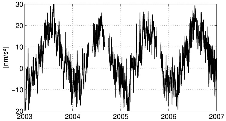
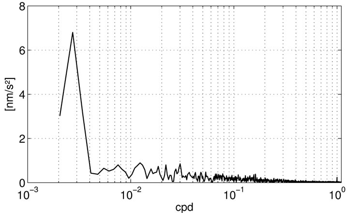
Figure 3. Difference between the attraction effects from the local zone, calculated from 3D data and 2D data for Membach (3D - 2D). Bottom: Corresponding Fourier amplitude spectrum.
reduction the scatter of the SCG residuals decreased. Considering the SCG residuals as random deviations, for uncorrelated observations it can be assumed, that an interfering disturbance with a scatter of 3.8 nm/s2  was removed from the SCG data. Relating this noise signal to SCG data (RMS: 25 nm/s2) the ECMWF based reduction improved the gravity observations by 15% compared to the classical method. The differences between both reduction methods are shown in Figure 4 and vary between −14 nm/s2 and +17 nm/s2 with an RMS of 5 nm/s2.
4. Atmospheric Reductions for FG5-220 Absolute Gravity Measurements in Fennoscandia
The individual contributions of attraction and deformation effects from the local, regional, and global zones have been derived using atmospheric 2D data. Additionally, the attraction effect from the local zone was also determined from 3D data, cf. Section 2. The inverse barometer hypothesis (IB) is applied for the reaction of the ocean to barometric pressure changes. Similar reduction results as shown in Table 1 are also obtained for absolute gravity measurements. From the local zone an extreme value of about 100 nm/s2 is obtained. The two other zones contribute each with about −11 nm/s2. The total ef-
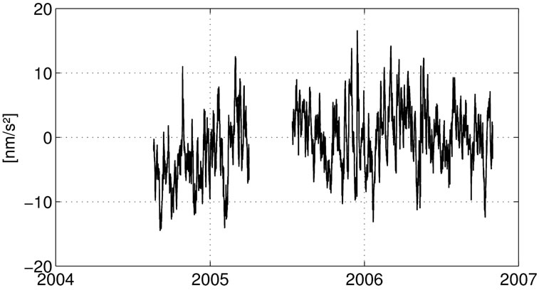
Figure 4. Difference between SCG series after applying classical barometric reduction and the ECMWF data based reduction.
fects from all zones vary between −71 nm/s2 and +73 nm/s2 with an RMS average of +27 nm/s2 and a mean value of 1 nm/s2.
Differences between gravity effects using ECMWF 2D and 3D data and the classical regression coefficient method are shown in Figure 5. One circle depicts the atmospheric gravity for each station determination with the Hannover absolute gravimeter FG5-220. These reduction improvements reach −19 and +4 nm/s2 with an RMS of 8 nm/s2. The atmospheric gravity modeling improves the reductions by 15% to 30%.
5. Summary and Conclusions
In this study, gravity changes due to atmospheric mass redistributions are calculated. The results are applied to high-precision gravity data of superconducting gravimeter in Membach and to absolute observations in the Fennoscandia with FG5-220. The used method is based on globally distributed ECMWF weather data, whereby the globe was divided into three zones around the computation point (gravity station): local, regional, and global zone. The atmospheric gravity effects (attraction and deformation) from all three zones were computed using Green’s functions and ECMWF 2D surface data. Additionally, the direct attraction effect from the local zone was determined directly using Newton’s law of gravity and ECMWF 3D data.
The modeling was verified with gravity data of the superconducting gravimeter in Membach. The residuals were improved by about 15% compared to the classical air pressure reduction with the standard regression coefficient  nm/s2 per hPa. For time series in Membach, the differences between both methods (improvements) vary between −14 and +17 nm/s2 with an RMS of 5 nm/s2. The seasonal vertical redistribution within a column of atmosphere (mass centre moves up in spring and down in fall) causes air pressure independent gravity attraction up to 50 nm/s2 (peak to peak) with an RMS of about 10 nm/s2. Also the effect from the global zone
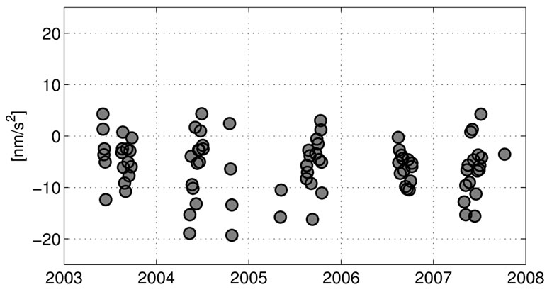
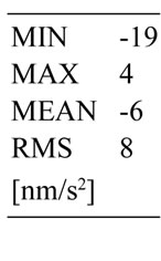
Figure 5. Differences between gravity effects derived from ECMWF 3D and 2D data, and from local pressure measurements (classic method with α = −3 nm/s2 per hPa) for absolute gravity station determinations with FG5-220 in Fennoscandia (2003- 2007).
contributes with about 10 nm/s2, which is not considered by the classical air pressure reduction using only local air pressure observations. The station air pressure is not correlated with the global contribution. For absolute gravity measurements with FG5-220 in Fennoscandia the atmospheric reduction improvements reach 20 nm/s2 with a mean variation of 8 nm/s2.
To identify subtle tectonic changes of secular character by gravimetry, a reduction accuracy of 3 nm/s2 is demanded. Therefore, the atmospheric gravity reduction should be modeled globally using 2D and 3D weather data for high-precision gravity observations.
6. Acknowledgements
Within the R & D-Programme GEOTECHNOLOGIEN this study was funded by the German Ministry of Education and Research (BMBF) and the German Research Foundation (DFG), Grant Mu 1141/3-1 and 3-2. We acknowledge support by Deutsche Forschungsgemeinschaft and Open Access Publishing Fund of Leibniz Universität Hannover. We like to thank the University of Cologne for providing ECMWF (European Centre for MediumRange Weather Forecasts) data in cooperation with the Deutsches Klimarechenzentrum (DKRZ). Thanks to Michel Van Camp for providing the superconducting gravity data. Steven S. Pietrobon is acknowledged for the software for the US Standard Atmosphere, 1976. Thanks to all involved colleagues from the Fennoscandian project partners for the fruitful cooperation: Federal Agency for Cartography and Geodesy (BKG, Frankfurt, Germany), Finnish Geodetic Institute (FGI, Masala, Finland), Lantmäteriet, Swedish mapping, cadastral and land registration authority (Gävle, Sweden), Onsala Space Observatory, Chalmers Univ. of Technology (Sweden), Statens Kartverk (Honefoss, Norway), Department of Mathematical Sciences and Technology, University of Environmental and Life Sciences (Ås, Norway), National Space Institute, Technical University of Denmark (DTU Space, Copenhagen, Denmark), Maa-amet, Estonian Land Board (Tallinn, Estonia).
REFERENCES
- L. Timmen, O. Gitlein, V. Klemann and D. Wolf, “Observing Gravity Change in Fennoscandian Uplift Area with the Hannover Absolute Gravimeter, Deformation and Gravity Change: Indicators of Isostasy, Tectonics, Volcanism and Climate Change,” Pure and Applied Geophysics, Vol. 169, No. 8, 2012, pp. 1331-1342. doi:10.1007/s00024-011-0397-9
- O. Gitlein, L. Timmen, J. Müller, H. Denker, J. Mäkinen, M. Bilker-Koivula, B. Pettersen, D. Lysaker, J. Svendsen, H. Wilmes, R. Falk, A. Reinhold, W. Hoppe, H.-G. Scherneck, B. Engen, O. Omang, A. Engfeldt, M. Lilje, G. Strykowski and R. Forsberg, “Observing Absolute Gravity Acceleration in the Fennoscandian Land Uplift Area,” Terrestrial Gravimetry: Static and Mobile Measurements (TG-SMM2007), International Symposium, Elektropribor, St. Petersburg, 20-23 August 2007, pp. 175-180.
- J. Ågren and R. Svensson, “Land Uplift Model and System Definition for the RH 2000 Adjustment of the Baltic Levelling Ring,” The 15th General Meeting of the Nordic Geodetic Commission, Copenhagen, 29 May-2 June 2006.
- M. Ekman and J. Mäkinen, “Recent Postglacial Rebound, Gravity Change and Mantle Flow in Fennoscandia,” Geophysical Journal International, Vol. 126, No. 1, 1996, pp. 229-234. doi:10.1111/j.1365-246X.1996.tb05281.x
- O. Gitlein, “Absolutgravimetrische Bestimmung der Fennoskandischen Landhebung mit dem FG5-220,” PhD Thesis, Wissenschaftliche Arbeiten der Fachrichtug Geodäsie und Geoinformatik der Leibniz Universität Hannover, 2009.
- O. Gitlein and L. Timmen, “Atmospheric Mass Flow Reduction for Terrestrial Absolute Gravimetry in the Fennoscandian Land Uplift Network,” Dynamic Planet, IAG Symposium, Cairns, 22-26 August 2005, pp. 461-466.
- R. J. Warburton and J. M. Goodkind, “The Influence of Barometricpressure Variations on Gravity,” Geophysical Journal International, Vol. 48, No. 3, 1977, pp. 281-292.
- T. M. van Dam and J. M. Wahr, “Displacements of the Earth’s Surface Due to Atmospheric Loading: Effects on Gravity and Baseline Measurements,” Journal of Geophysical Research, Vol. 92, No. B2, 1987, pp. 1281-1286. doi:10.1029/JB092iB02p01281
- T. M. van Dam, G. Blewitt and M. B. Heflin, “Atmospheric Pressure Loading Effects on Global Positioning System Coordinate Determinations,” Journal of Geophysical Research, Vol. 99, No. B12, 1994, pp. 23939-23950. doi:10.1029/94JB02122
- H.-P. Sun, “Static Deformation and Gravity Changes at the Earth’s Surface due to the Atmospherical Pressure,” PhD Thesis, Catholic University of Louvain, Belgium, 1995.
- C. Kroner, “Reduktion von Luftdrucke_ekten in Zeitabhängigen Schwerebeobachtungen,” PhD Thesis, Mathematisch-Naturwissenschaftliche Fakultät, Technische Universität Clausthal, 1997.
- J.-P. Boy, P. Gegout and J. Hinderer, “Reduction of Surface Gravity Data from Global Atmospheric Pressure Loading,” Geophysical Journal International, Vol. 149, No. 2, 2002, pp. 534-545. doi:10.1046/j.1365-246X.2002.01667.x
- L. Petrov and J.-P. Boy, “Study of the Atmospheric Pressure Loading Signal in Very Long Baseline Interferometry Observations,” Journal of Geophysical Research, Vol. 109, 2004, Article ID: B03405. doi:10.1029/2003JB002500
- D. Crossley, J. Hinderer and J.-P. Boy, “Regional Gravity Variations in Europe from Superconducting Gravimeters,” Journal of Geodynamics, Vol. 38, No. 3-5, 2004, pp. 325-342. doi:10.1016/j.jog.2004.07.014
- D. Bock, R. Noomen and H.-G. Scherneck, “Atmospheric Pressure Loading Displacement of SLR Stations,” Journal of Geodynamics, Vol. 39, No. 3, 2005, pp. 247-266. doi:10.1016/j.jog.2004.11.004
- P. Tregoning and T. M. van Dam, “Atmospheric Pressure Loading Corrections Applied to GPS Data at the Observation Level,” Geophysical Research Letters, Vol. 32, 2005, Article ID: L22310. doi:10.1029/2005GL024104
- T. Klügel and H. Wziontek, “Correcting Gravimeters and Tiltmeters for Atmospheric Mass Attraction Using Operational Weather Models,” Journal of Geodynamics, Vol. 48, No. 3-5, 2009, pp. 204-210. doi:10.1016/j.jog.2009.09.010
- M. Abe, C. Kroner, J. Neumeyer and X. Chen, “Assessment of Atmospheric Reductions for Terrestrial Gravity Observations,” Bulletin d’Information des Marées Terrestres, Vol. 146, 2010, pp. 11817-11838.
- H. Häckel, “Meteorologie,” Eugen Ulmer KG, Stuttgart, 2005.
- I. M. Longman, “A Green’s Function for Determining the Deformation of the Earth under Surface Mass Loads: 1. Theory,” Journal of Geophysical Research, Vol. 67, No. 2, 1962, pp. 845-850. doi:10.1029/JZ067i002p00845
- W. E. Farrell, “Deformation of the Earth by Surface Loads,” Reviews of Geophysics and Space Physics, Vol. 10, No. 3, 1972, pp. 761-797.
- J. B. Merriam, “Atmospheric Pressure and Gravity,” Geophysical Journal International, Vol. 109, No. 3, 1992, pp. 488-500. doi:10.1029/RG010i003p00761
- J. Y. Guo, Y. B. Li, Y. Huang, H. T. Deng, S. Q. Xu and J. S. Ning, “Green’s Function of the Deformation of the Earth as a Result of Atmospheric Loading,” Geophysical Journal International, Vol. 159, No. 1, 2004, pp. 53-68. doi:10.1111/j.1365-246X.2004.02410.x
- R. S. Spratt, “Modelling the Effect of Atmospheric Pressure Variations on Gravity,” Geophysical Journal International, Vol. 71, 1982, pp. 173-186.
- S. R. Dickman, “Theoretical Investigation of the Oceanic Inverted Barometer Response,” Journal of Geophysical Research, Vol. 93, No. B12, 1988, pp. 14941-14946. doi:10.1029/JB093iB12p14941
- C. Wunsch and D. Stammer, “Atmospheric Loading and the Oceanic ‘Inverted Barometer’ Effect,” Reviews of Geophysics, Vol. 35, No. 1, 1997, pp. 79-107. doi:10.1029/96RG03037
- T. M. van Dam and J. M. Wahr, “The Atmopsheric Load Response of the Ocean Determined Using Geosat AlTimeter data,” Geophysical Journal International, Vol. 113, No. 1, 1993, pp. 1-16.
- W. Rabbel and J. Zschau, “Static Deformation and Gravity Changes at the Earth’s Surface Due to Atmospheric Loading,” Journal of Geophysics, Vol. 56, 1985, pp. 81- 99.
- H.-P. Sun, B. Ducarme and V. Dehant, “Effect of the Atmospheric Pressure on Surface Displacements,” Journal of Geodesy, Vol. 70, No. 3, 1995, pp. 131-139. doi:10.1007/BF00943688
- J. Johansson, J. Davis, H.-G. Scherneck, G. Milne, M. Vermeer, J. Mitrovica, R. Bennett, B. Jonsson, G. Elgered, P. Elósegui, H. Koivula, M. Poutanen, B. Rönnäng and I. Shapiro, “Continuous GPS Measurements of Postglacial Adjustment in Fennoscandia, 1. Geodetic Results,” Journal of Geophysical Research, Vol. 107, No. B8, 2002, pp. 1-27. doi:10.1029/2001JB000400
- H.-G. Scherneck, J. Johansson, H. Koivula, T. van Dam and J. Davis, “Vertical Crustal Motion Observed in the BIFROST Project,” Journal of Geodynamics, Vol. 35, No. 4-5, 2003, pp. 425-441. doi:10.1016/S0264-3707(03)00005-X
- IGC, “International Absolute Gravity Basestation Network (IAGBN), Absolute Gravity Observations, Data Processing, Standards & Station Documentation (Int. Grav. Com.—WGII: World Gravity Standards),” Bureau Gravimetrique International, Bulletin d’Information, Vol. 63, 1988, pp. 51-57.
- D. Simon, “Modelling of the Gravimetric Effects Induced by Vertical Air Mass Shifts,” In: Mitteilungen des Bundesamtes für Kartographie und Geodäsie, Verlag des Bundesamtes für Kartographie und Geodäsie, Frankfurt am Main, 2003.
- J. Neumeyer, J. Hagedoorn, J. Leitloff and T. Schmidt, “Gravity Reduction with Three-Dimensional Atmospheric Pressure Data for Precise Ground Gravity Measurements,” Journal of Geodynamics, Vol. 38, 2004, pp. 437-450. doi:10.1016/j.jog.2004.07.006
- M. Talwani and M. Ewing, “Rapid Computation of Gravitational Attraction of Three-Dimensional Bodies of Arbitrary Shape,” Geophysics, Vol. 25, No. 1, 1960, pp. 203-225. doi:10.1190/1.1438687
- K. Jung, “Schwerkraftverfahren in der Angewandten Geophysik,” Geest & Portig K.-G., Leipzig, 1961.
- D. Nagy, “The Gravitational Attraction of a Right Rectangular Prism,” Geophysics, Vol. XXXI, No. 2, 1966, pp. 362-371. doi:10.1190/1.1439779
- H. Buitkamp, “Modelle für Geodätische Anwendungen der Trägheitsnavigation mit Besonderer Berücksichtigung von Schachtvermessungen,” Dissertation, Verö_entlichungen der Deutschen Geodätischen Kommission bei der Bayerischen Akademie der Wissenschaften, Reihe C, Nr. 306, Rheinische Friedrich-Wilhelms-Universität zu Bonn, München, 1960.
- D. Nagy, G. Papp and J. Benedek, “The Gravitational Potential and Its Derivatives for the Prism,” Journal of Geodesy, Vol. 74, No. 7, 2000, pp. 552-560. doi:10.1007/s001900000116
- H. Kraus, “Die Atmosphäre der Erde: Eine Einführung in die Meteorologie,” Springer, Berlin, 2004.
- J. M. Goodkind, “The Superconducting Gravimeter,” Review of Scientific Instruments, Vol. 70, No. 11, 1999, pp. 4131-4152. doi:10.1063/1.1150092
- O. Francis, M. Van Camp, T. van Dam, R. Warnant and M. Hendrickx, “Indication of the Uplift of the Ardenne in Long Term Gravity Variations in Membach (Belgium),” Geophysical Journal International, Vol. 158, No. 1, 2004, pp. 346-352.
- M. Van Camp, M. Vanclooster, O. Crommen, T. Petermans, K. Verbeek, B. Meurers, T. M. van Dam and A. Dassargues, “Hydrogeological Investigations at the Membach Station, Belgium, and Application to Correct Long Periodic Gravity Variations,” Journal of Geophysical Research, Vol. 111, 2006, Article ID: B10403. doi:10.1029/2006JB004405