Journal of Flow Control, Measurement & Visualization
Vol.1 No.2(2013), Article ID:34552,16 pages DOI:10.4236/jfcmv.2013.12006
A Comparison Study of Cavitating Flow in a Ventricular Assist Device Using Laminar and Turbulent Model*
National Taiwan Ocean University, Keelung, Taiwan
Email: #b0105@mail.ntou.edu.tw
Copyright © 2013 Chengkuo Huang, Jiahn-Horng Chen. This is an open access article distributed under the Creative Commons Attribution License, which permits unrestricted use, distribution, and reproduction in any medium, provided the original work is properly cited.
Received November 27, 2012; revised January 25, 2013; accepted February 20, 2013
Keywords: Cavitation; Ventricular Assist Device; Valve; Turbulent Flow; Laminar Flow
ABSTRACT
The two-dimensional cavitating flow phenomena due to the valve closure in a ventricular assist device were computationally studied. This is a simplification of three-dimensional viscous effects in a ventricular valve. Both laminar flow and turbulent flow were computed and compared with each other. For computations, a dynamic mesh strategy to cope with the movement of the valve was developed. The simulation of cavitation was conducted with a model which took considerations of the first-order effect of the formation and transport of vapor bubbles, the turbulent fluctuations of pressure and velocity, and the magnitude of non-condensable gases. The turbulent flow was computed by using the k-w model. The results show that the local turbulence is one of the vital effects on the development of the cavitating flow. The maximum velocity at the moments of valve closure was significantly reduced in the turbulent flow modeling. Turbulence also reduces the jet intensity at the valve closure and, hence, the cavitating region on the valve. Furthermore, the results show that the turbulent flow model has a better capability for prediction of cavitation duration.
1. Introduction
Cavitation was first related to valves of a mechanical heart in the 1980s after a series of valve fractures of a particular valve were observed [1]. Since then, many experimental and computational efforts have been devoted to understanding the flow and its detrimental effects on long-term operations of ventricular assist devices or artificial hearts. It has been known that cavitation could result in damage of blood cells and, hence, increase the risk of thromboembolic complications found in patients implanted with a mechanical heart. Various techniques for in vivo and/or in vitro detection of cavitation have been developed in the past few decades [2-6]. From the physical point view, such cavitating phenomena arises partially due to the fact that the pressure surge and the water hammer effect happen in closing ventricular valve (see, e.g., [7]). The drastic transient pressure change resulted from the pressure surge makes the cavitation even worse and more complicated.
In addition to various physiological issues, many physical phenomena due to mechanical heart valve closure have also been studied experimentally. Wu et al. [8] developed a laser sweeping technique which was capable of monitoring the valve closing motion with microsecond precision. Their observations show that at valve closure, the water hammer pressure reduction in combination with the high energy squeeze jet formed an environment favoring micro cavitation inceptions. Lee et al. [9] studied cavitation dynamics for different mechanical mitral heart valves using a stroboscopic visualization technique. Their in vitro study revealed several sources of cavitation initiation, including occluder stop, inflow strut, and clearance. They also concluded that the effects of fluid squeezing and the streamline contraction are major factors inducing cavitation incipience. Biancucci et al. [10] used a mock circulatory loop and videotaped the valve motion and the fluid flow around it. They found that gas bubbles formed during valve operation in the low pressure region due to gaseous nuclei and the presence of CO2. More recently, the high density particle image velocimetry technique has been developed. Detailed flow description becomes possible. It was found that the rebound effect played a significant role in the cavitation formation [11]. Lim et al. [12] further employed the high-speed flow imaging technique to identify regions of cavitation and found that the temporal fluid acceleration played an important role on cavitation inception. All these findings provide important inferences in the design of mechanical heart valves.
With the advancement of computational fluid dynamics (CFD), the numerical simulation has become an important strategy in the industrial design process for verifying and validating new product designs. This is no exception in the design of mechanical heart valves and ventricular assist devices. Makhihani et al. [13] specified the valve closing motion which was measured in vitro as input data and used a CFD package to compute the flow field. They predicted the possibility of cavitation inception by observing whether the fluid pressures dropped below the blood saturated vapor pressure. Lai et al. [14] employed CFD model to analyze the valve closure process and successfully evaluated the effect of alternations in the valve tip geometry. They concluded that a decrease of the tip velocity in the last few degrees led to a significant reduction of the negative pressure magnitude and, hence, the possibility of cavitation. Later, Cheng et al. [15] extended the CFD study to three-dimensional cases and observed vertical flow development during the valve impact-rebound phase.
It is quite unfortunate that most computational studies were restricted to laminar flow simulations though it is well known that cavitation usually happens in a highspeed region where the flow is usually turbulent. Furthermore, the inception of cavitation is usually indirectly inferred by observing whether the pressure drops below the saturated vapor pressure. In fact, it is vital to develop turbulent flow computation strategies with more realistic cavitation models to cope more rigorously with the medical physical phenomenon. Recently, Huang and Chen [16] first proposed a k-w turbulent model and employed a more realistic cavitation model to analyze the cavitation inception and process during the valve closure. The computed cavitation time endurance agrees with that available in the literature. In the present study, we applied the similar strategy to simulate the flow of a mechanical heart valve closure and compared the results obtained by laminar and turbulent models.
2. Physical Problem
Shown in Figure 1, a two-dimensional bileaflet valve system in a channel is analyzed in the present study. The length and width of the channel is L and 2w, respectively. Point O is the pivot of the valve. The lengths from both valve ends to the pivot is  and
and , respectively. The gauge pressure variations at the inlet and outlet are specified as
  and
and , respectively. The angular position of valve is given by
 .
.
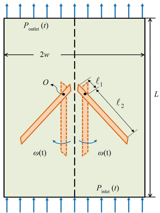
Figure 1. Physical domain of the problem.
Considering the cavitating effects, the two-dimensional governing equations can be expressed as
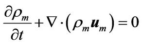 (1)
(1)
and
 (2)
(2)
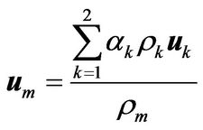
where  and
and  are the mixed density and velocity defined as
 (3)
(3)
( represents the volume fraction of phase k = 1 and 2 for liquid and gas phase, respectively) and
 (4)
(4)
respectively. Furthermore, p denotes the pressure and  the mixed viscosity
 (5)
(5)
The drift velocity
 (6)
(6)
To find the fluid velocities and densities of liquid and gas phases, we employed the full cavitation model proposed by Singhal et al. [17]. This model employs a homogeneous flow approach and assumes that there are plenty nuclei for the cavitation inception. The following first-order effects are considered: the formation and transport of vapor bubbles, the turbulent fluctuations of pressure and velocity, and the magnitude of non-condensable gases. In the model, the phase-change vapor pressure is taken at
 (7)
(7)
where  is the saturation pressure of liquid and
 ![]() the turbulent pressure fluctuations
the turbulent pressure fluctuations
 (8)
(8)
with k being denoted the turbulent kinetic energy. The bubble growth and collapse is considered with the assumption of a zero velocity slip between fluid and bubbles. In addition, we also assume that the flow is isothermal and the fluid properties are constant in the whole flow domain. This implies that the cavitation is decoupled from heat transfer and radiation. For further elaboration of the bubble dynamics, please refer to [17].
Furthermore, to take account of the local turbulent flow effect, we used the k-w turbulence model which is more suitable to model turbulent flow at a smaller Reynolds number. The model employed in the present study is based on the results of Wilcox [18]. It is applicable to wall-bounded flows. For further elaboration of the equation systems taking cavitation into considerations, please refer to [16].
As shown in the governing equations, Equations (1) and (2), the mixture model is employed in the present study. The local velocity and density are functions of the volume fraction of vapor phase which is, in turn, controlled by the cavitation model through the bubble dynamics equation. Therefore, the local transition from laminar to turbulent flow can be influenced by the presence of cavitation. The interaction between the transition and cavitation is complicated and determined by the turbulence model, cavitation model, and the flow governing equations. Such an interaction could be an interesting fundamental issue but is beyond the present scope of study.
3. Numerical Method and Mesh Strategy
The commercial code FLUENT (version 6.3) was employed for the present study. In the code, the finite volume method was employed to discretize all differential equations and the algorithm of pressure implicit with splitting of operators (PISO) was adopted for nonlinear iterations of pressure and velocity solutions. The PISO algorithm is efficient and more accurate to solve the Navier-Stokes equations in unsteady problems because the momentum corrector step is performed more than once, compared to the traditional SIMPLE algorithm. The numerical procedures to compute the laminar and turbulent flows are identical except that the latter employed a turbulence model.
In the present study, the valve moves in time from a vertical position to a horizontal one. To cope with the motion, we employed a local dynamic mesh strategy which combines the spring-smoothing method and the local remeshing method. Shown in Figure 2, we divided the computational domain into three regions. In the regions away from and around the valve, a structured cartesian mesh was employed. The reason we used a structured grid around the valve is that it ensures better grid orthogonality and, hence, better solution quality in the region near the valve. In the region where the valve motion occurs, a non-structured mesh was generated.
With the valve motion, the mesh must be regenerated at each time step. However, since in computations, the time step is usually very small, it is not necessary to
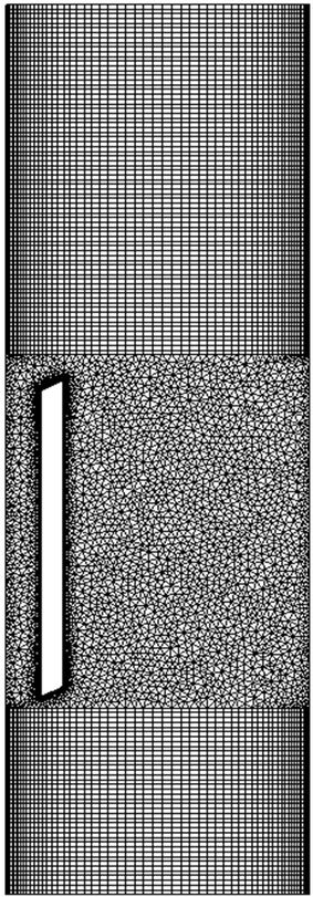

Figure 2. Mesh strategy.
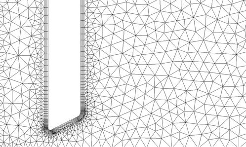
remesh at every time step. Rather, we employed the spring-smoothing method to stretch and/or compress the local mesh near the valve in several consecutive time steps. When the local mesh becomes severely distorted, we remesh the grids around the valve. The grids near the valve at different times are shown in Figure 3.
4. Results and Discussions
In the following study, the geometric data we used for analysis are L = 38.1mm, w = 12.21 mm,  mm, and
  mm. The densities for liquid and gas are
  kg/m3 and
  kg/m3, respectively. Furthermore, their dynamic viscosities are
  kg/m×sec and
  kg/m×sec, respectively.
For comparison purposes, the specification of the inlet and outlet pressures and the valve rotation follows that in [14]. The inlet pressure  increases at a rate of 2 mmHg/ms from zero at t = 0 sec till it reaches 120 mmHg. The outlet pressure
  keeps at zero for all time. The valve is at its vertical position at t = 0 sec as shown in Figure 2 and rotates at a rate specified in [14].
After several tests, the appropriate time step is 
 sec. However, for a better resolution of cavitation phenomena, we require that
  sec.
sec.
4.1. Velocity Distribution before Cavitation
Figures 4 and 5 show the velocity distributions at different values of t for both the laminar and turbulent models, respectively. Due to the turbulence viscosity in the turbulent model, it is expected that the maximum velocity is significantly reduced in the turbulent flow simulation. Table 1 shows the maximum speed in the flow field at some particular time.
Figure 6 shows the maximum value variation of k with respect to time when we employed the turbulent flow model. Evidently, the flow is laminar at time t < 0.015 sec. Due to the increase of velocity, the flow begins to exhibit turbulent characteristic during 0.015 sec <
 (a)
(a)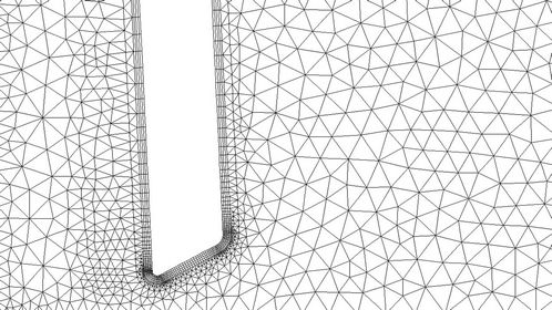 (b)
(b)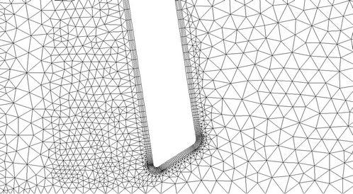 (c)
(c)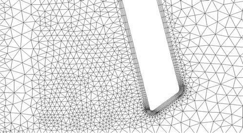 (d)
(d)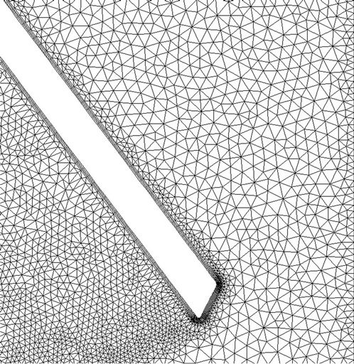 (e)
(e)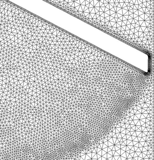 (f)
(f)
Figure 3. Mesh near the valve at different locations of valve. (a) t = 0.00 sec; (b) t = 0.01 sec; (c) t = 0.02 sec; (d) t = 0.024 sec; (e) t = 0.03 sec; (f) t = 0.0324 sec.
 (a)
(a)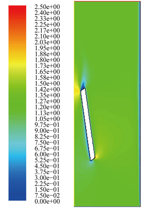 (b)
(b)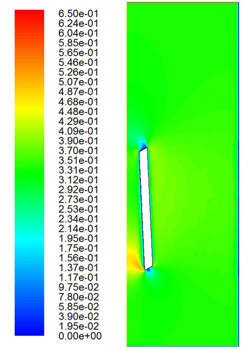 (c)
(c) (d)
(d) (e)
(e)
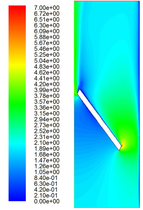
Figure 4. Velocity distributions with the laminar model. (a) t = 0.01 sec; (b) t = 0.02 sec; (c) t = 0.03 sec; (d) t = 0.0315 sec; (e) t = 0.0324 sec.
t < 0.03 sec. And for t > 0.03 sec, the flow becomes locally turbulent. And it is evident that k increases drastically after t > 0.0324 sec when the cavitation occurs near the valve tip which will be further discussed later in Section 4.2. This implies that the turbulent effects are important when we investigate the flow cavitation.
4.2. Cavitation
The time-variations of maximum volume fraction in gas phase and the minimum pressure in the computational domain are shown in Figures 7 and 8, respectively. They are both proper indicators of cavitation. It is a common practice in the literature to specify that cavitation occurs when . According to the computational results shown in these two figures, it is interesting to find that cavitation occurs almost at the same time in laminar and turbulent computations (t = 0.0324 sec). Nevertheless, the duration of cavitation is much longer in the laminar flow computation than in the turbulent flow computations. The former is about 670 msec and the latter about 550 msec which agrees with the measured data in [14]. This implies that consideration of turbulent effects leads to a better prediction, as far as the cavitation duration is concerned.
 (a)
(a)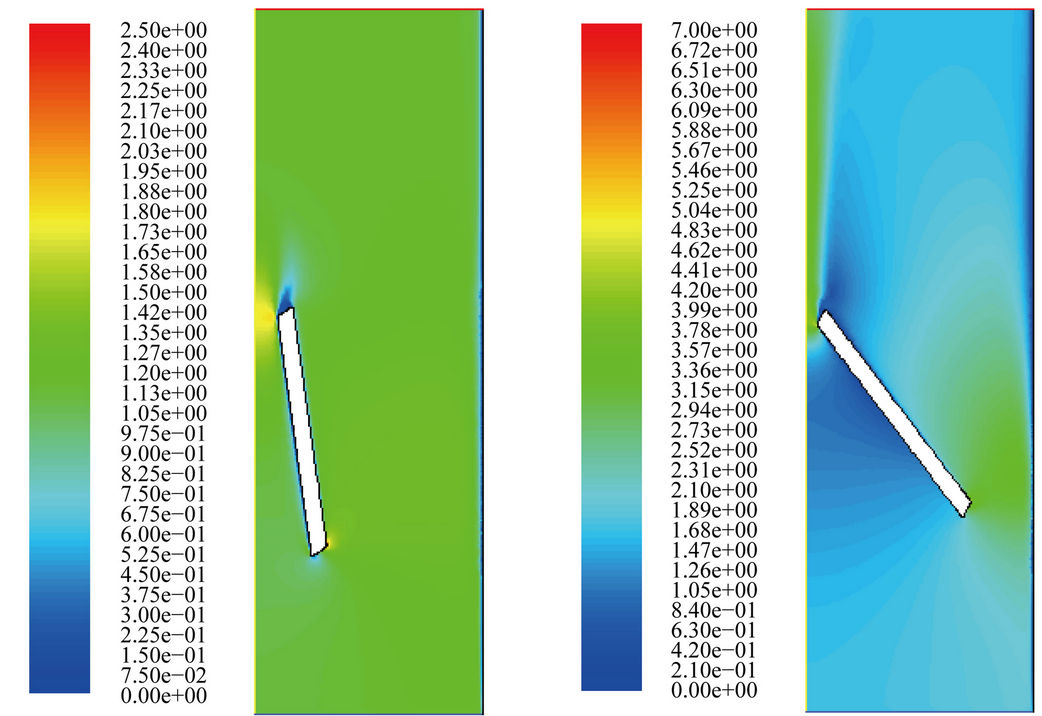 (b)
(b)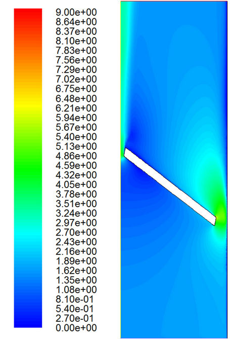 (c)
(c)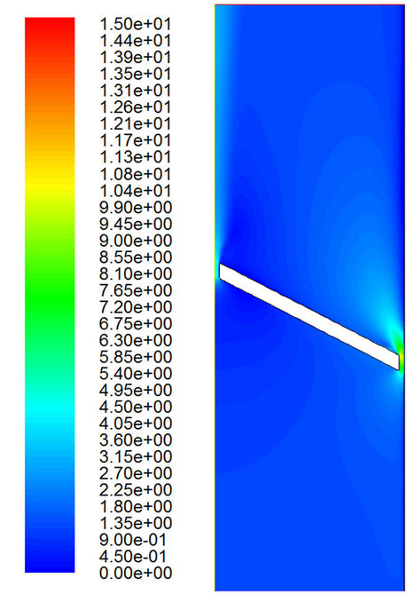 (d)
(d)
Figure 5. Velocity distributions with the turbulent model. (a) t = 0.01 sec; (b) t = 0.02 sec; (c) t = 0.03 sec; (d) t = 0.0315 sec; (e) t = 0.0324 sec.
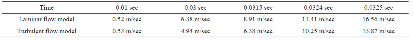
Table 1. Maximum speed for different flow models.
4.3. Pressure and Velocity Distributions during Cavitation
Figures 9 and 10 show the pressure distributions during the period of cavitation. The major difference for different models appears in the small region near the valve tip. Obviously, the low-pressure region (dark blue area) on the outlet side is much bigger for the laminar flow model than that for the turbulent flow model. Furthermore, it is interesting to find that the low pressure first appears in the region near the tip of the valve. Then it seems to propagate very quickly downstream and disappear gradually far downstream. Of course, the low pressure wave propagates far more downstream for the laminar flow model than that for the turbulent flow model. However, the pressure keeps its low value around the trailing edge on
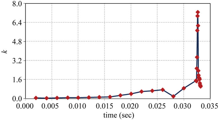
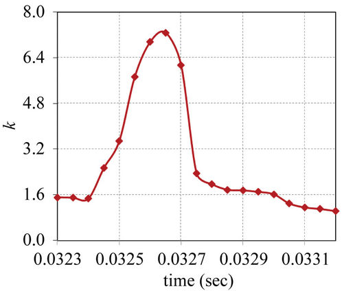
Figure 6. Variation of the maximum value of k.
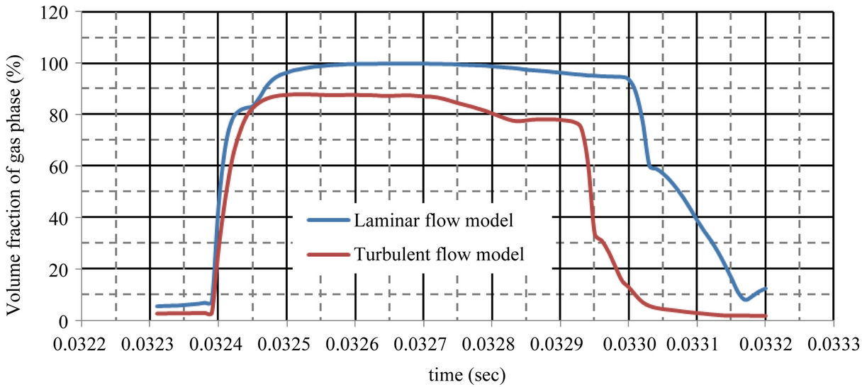
Figure 7. Maximum volume fraction of gas phase for different flow models.
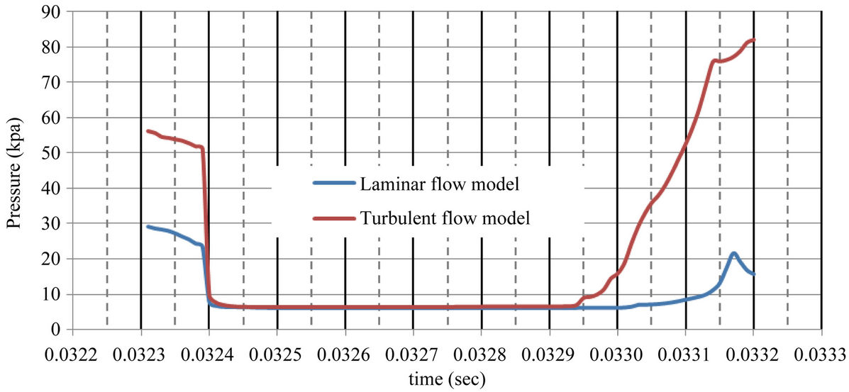
Figure 8. Minimum pressure variation for different flow models.
the tip during the period of cavitation for both models.
On the inlet side, the pressure distributions are almost the same for both models. This can be understood because the flow on this side is very small, as shown in Figures 11 and 12.
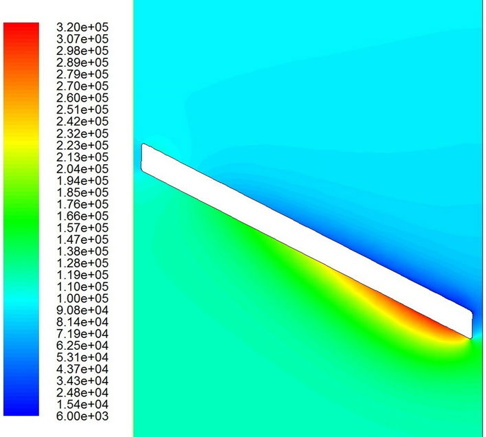
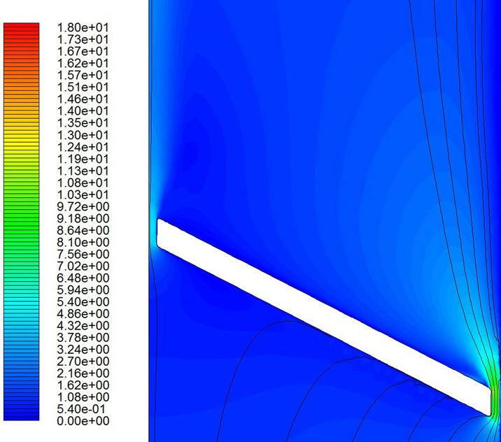
The speed variations in the flow field and the streamlines are shown in Figures 11 and 12. Again, the velocity is higher in the laminar flow simulation than that in the turbulent one. Of course, the highest velocity appears in the gap between the valve tip and the channel wall. The small gap induces a strong jet flow.
As the jet flow reduces its strength near the end of the valve motion, two vortical flows form at both valve tip regions. For the laminar flow model, the vortical flow on the right valve tip lasts longer. Meanwhile, the vortical flow on the left valve tip appears stronger for the turbulent flow model. Since the vortical flow implies that fluid particles in this region cannot move on, it is not a favor-
 (a)
(a)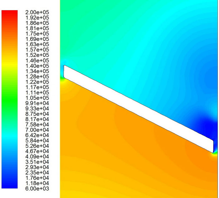 (b)
(b)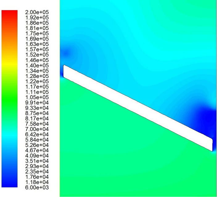 (c)
(c)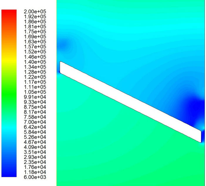 (d)
(d) (e)
(e)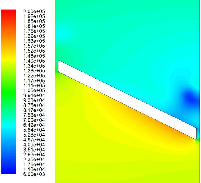 (f)
(f)
Figure 9. Pressure distributions with the laminar flow model. (a) t = 0.0324 sec; (b) t = 0.0326 sec; (c) t = 0.0328 sec; (d) t = 0.0329 sec; (e) t = 0.0330 sec; (f) t = 0.03316 sec.
 (a)
(a) (b)
(b)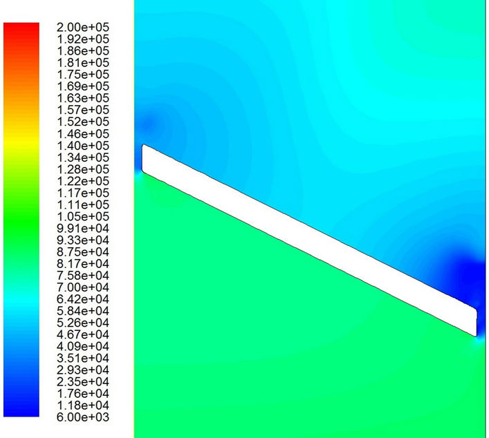 (c)
(c)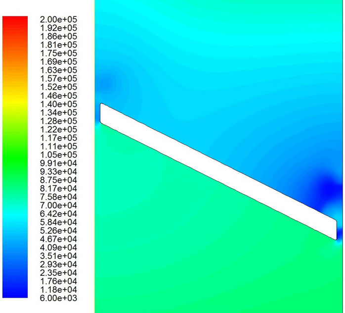 (d)
(d)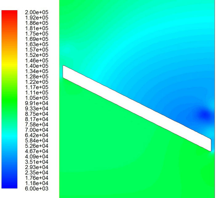 (e)
(e)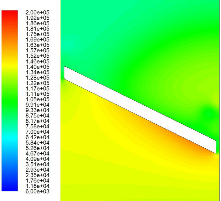 (f)
(f)
Figure 10. Pressure distributions with the turbulent flow model. (a) t = 0.0324 sec; (b) t = 0.0326 sec; (c) t = 0.0328 sec; (d) t = 0.0329 sec; (e) t = 0.0330 sec; (f) t = 0.03316 sec.
 (a)
(a)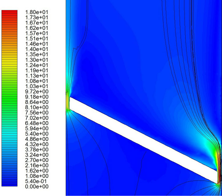 (b)
(b)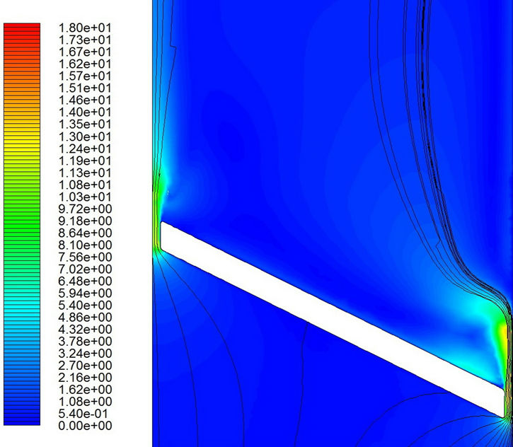 (c)
(c)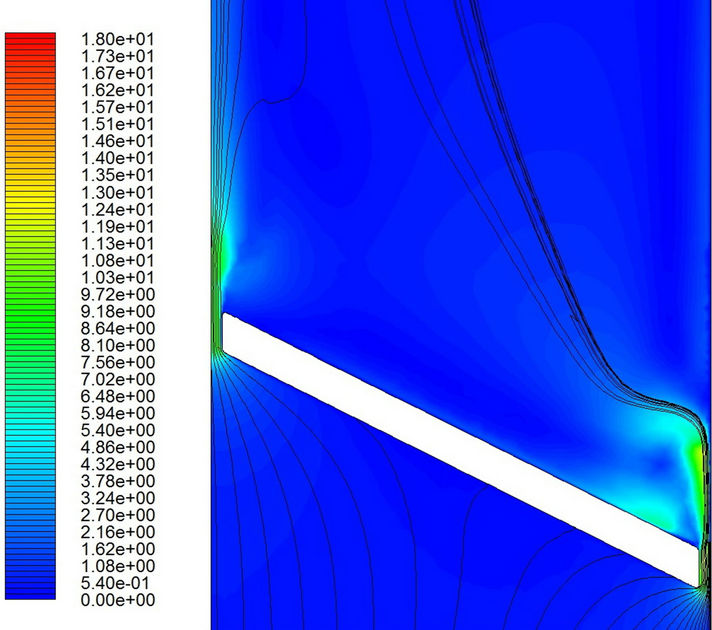 (d)
(d)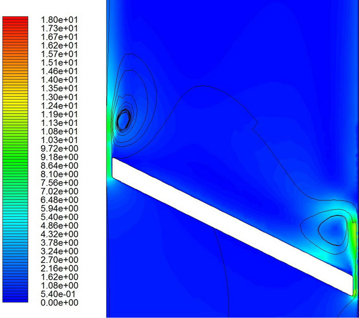 (e)
(e)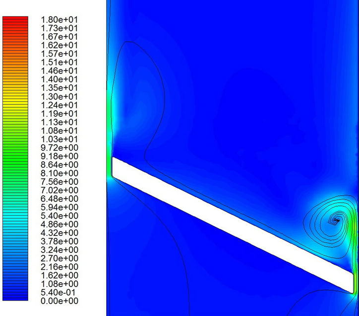 (f)
(f)
Figure 11. Velocity distributions and streamlines with the laminar flow model. (a) t = 0.0324 sec; (b) t = 0.0326 sec; (c) t = 0.0328 sec; (d) t = 0.0329 sec; (e) t = 0.0330 sec; (f) t = 0.03316 sec.
 (a)
(a) (f)
(f)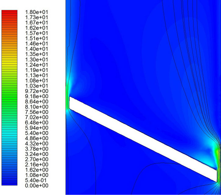 (c)
(c)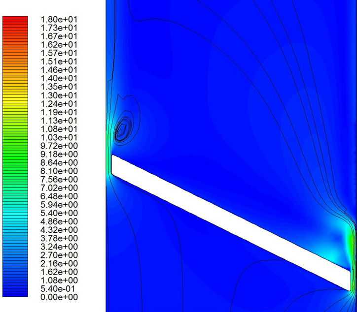 (d)
(d)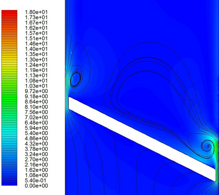 (e)
(e)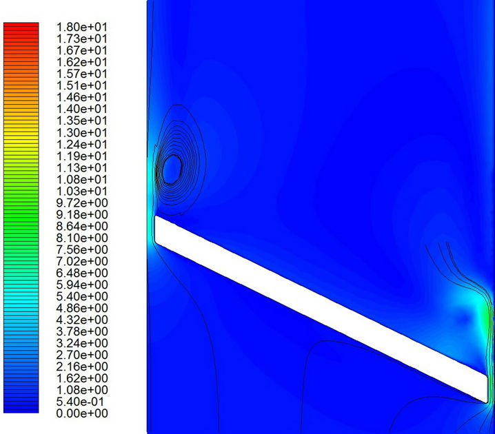 (f)
(f)
Figure 12. Velocity distributions and streamlines with the turbulent flow model. (a) t = 0.0324 sec; (b) t = 0.0326 sec; (c) t = 0.0328 sec; (d) t = 0.0329 sec; (e) t = 0.0330 sec; (f) t = 0.03316 sec.
able phenomenon and should be avoided.
4.4. Cavitation Bubble Variation
In terms of volume fraction of gas phase, the cavitation bubble evolution is shown in Figures 13 and 14. According to the previous discussions on pressure and velocity distributions, it is expected that the cavitation bubble is bigger and stronger for the laminar flow model.
 (a)
(a) (b)
(b)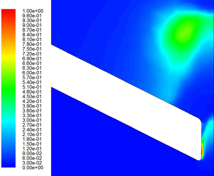 (c)
(c)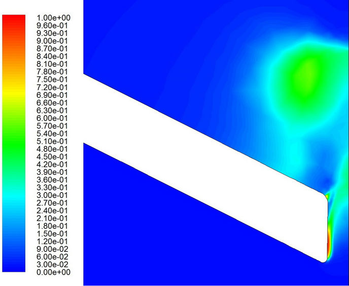 (d)
(d)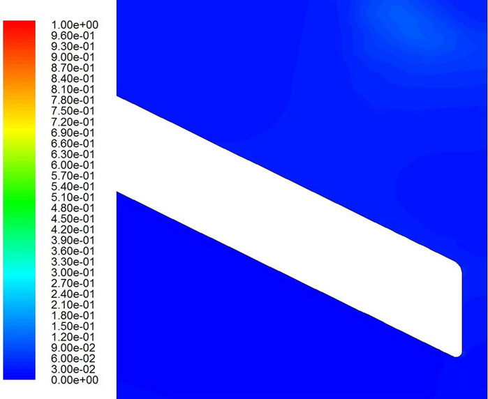 (e)
(e) (f)
(f)
Figure 13. Volume fraction of gas phase with the laminar flow model. (a) t = 0.0324 sec; (b) t = 0.0326 sec; (c) t = 0.0328 sec; (d) t = 0.0329 sec; (e) t = 0.0330 sec; (f) t = 0.03316 sec.
 (a)
(a) (b)
(b)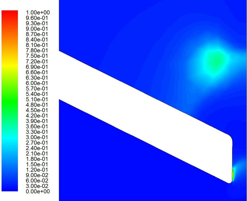 (c)
(c) (d)
(d)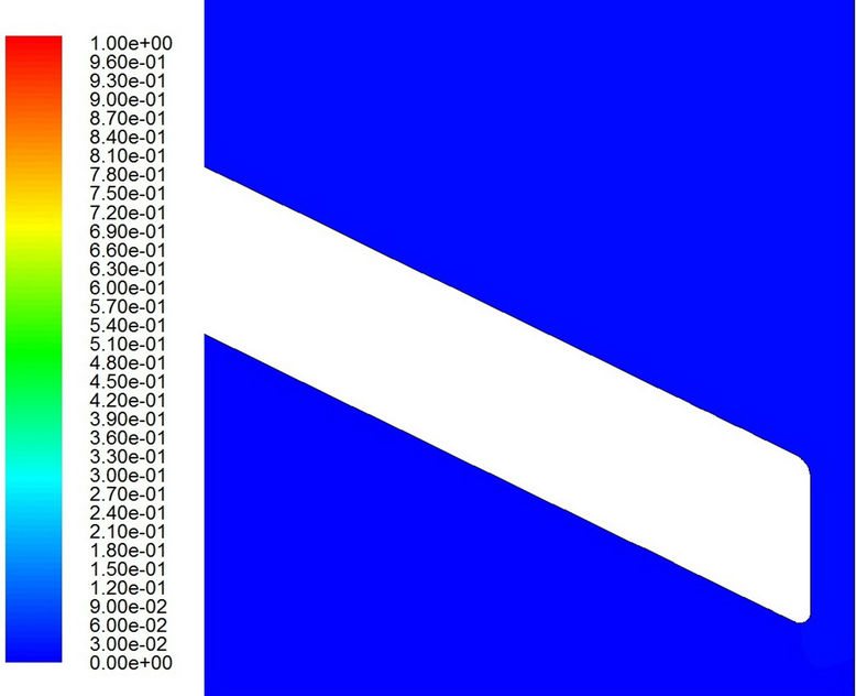 (e)
(e) (f)
(f)
Figure 14. Volume fraction of gas phase with the turbulent flow model. (a) t = 0.0324 sec; (b) t = 0.0326 sec; (c) t = 0.0328 sec; (d) t = 0.0329 sec; (e) t = 0.0330 sec; (f) t = 0.03316 sec.
Furthermore, it propagates farther downstream.
Nevertheless, in both models, the cavitation bubble first appears on the leading edge of the valve tip. Then it grows and moves along the valve surface on the downstream side, and later detaches from the valve and moves into the downstream flow field. In the meantime, another bubble appears on the trailing edge of the valve tip. Though it also grows as the first one, it collapses soon after its appearance. This could be due to the fact that the pressure recovers very soon at this stage. The first cavitation bubble which moves into the flow field shrinks in size and decays in strength at the same time. For the turbulent flow computation, it disappears not far downstream from the valve. Unfortunately, there are no detailed experimental data available to compare with the present computational results. However, as pointed out in the previous section, the cavitation duration computed from the turbulent flow model is consistent with that found in the experiment.
In the present study, the two important factors governing the growth and decay of cavitation bubbles for a specified saturation pressure are the local velocity and the turbulence intensity. The former enhances cavitation as its value is increased. The latter raises the phasechange threshold pressure due to the presence of turbulent pressure fluctuations which is proportionally related to the turbulence kinetic energy as shown in Equations (7) and (8). The two factors compete with each other to induce cavitation. The results in the present study show that the reduction of velocity due to the k-w turbulence model has a stronger effect than the production of turbulent kinetic energy. Hence, the results with the turbulent flow model show a shorter duration of cavitation event and smaller cavitation regions.
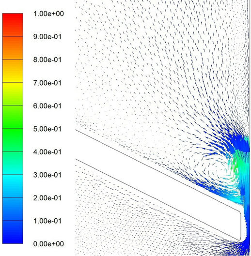
Finally, some comments are made for cavitation in separated regions. Shown in Figures 15 and 16 are the velocity vectors at different moments. The color in these figures represents the volume fraction of vapor phase. Evidently, a separated region appears on the downstream side beyond the valve for either laminar or turbulent flow model. A recirculating region is formed. Cavitation appears upstream of the reattachment zone. The results are
 (a)
(a) (b)
(b) (c)
(c)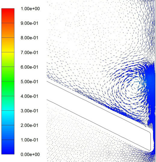 (d)
(d)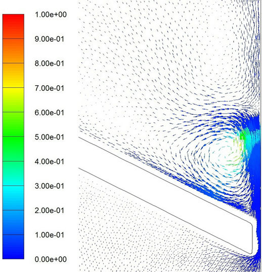 (e)
(e)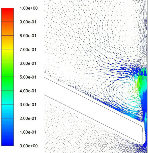 (f)
(f)
Figure 15. Velocity vector with colored volume fraction distribution of vapor phase for laminar flow model. (a) t = 0.0324 sec; (b) t = 0.0326 sec; (c) t = 0.0328 sec; (d) t = 0.0329 sec; (e) t = 0.0330 sec; (f) t = 0.03316 sec.
 (a)
(a) (b)
(b) (c)
(c) (d)
(d)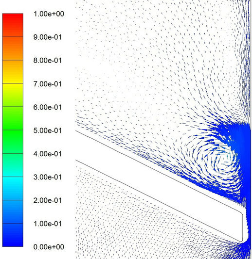 (e)
(e)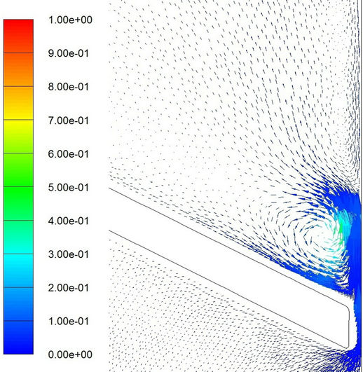 (f)
(f)
Figure 16. Velocity vector with colored volume fraction distribution of vapor phase for turbulent flow model. (a) t = 0.0324 sec; (b) t = 0.0326 sec; (c) t = 0.0328 sec; (d) t = 0.0329 sec; (e) t = 0.0330 sec; (f) t = 0.03316 sec.
similar to those observed by Katz [19]. Nevertheless, further elaboration is difficult (and beyond the scope of the present study) because of the employment of mixture model in computations because we did not consider nuclei population, the radius distribution, and the bubble dynamics in a microscopic point of view.
5. Conclusions
We have presented a comparison study of laminar and turbulent cavitating flow development due to a bileaflet valve motion in the ventricular assist device. For the turbulent flow simulation, the k-w model was employed since turbulence is a local effect which is significant only in the region near the valve tip.
The results show that the major difference in pressure and velocity fields from each other appears in the region near the valve tip of the long arm. However, the difference is significant only when t > 0.015 sec. When t < 0.015 sec, the flow is predominantly laminar throughout the flow field and there is almost no significant turbulent effect. However, for t > 0.015 sec, local turbulence near the valve tip becomes significant. Due to the turbulence viscosity, the maximum speed in the flow field is smaller for the turbulent model.
Since cavitation occurs in the region where the flow speed is high, turbulence is an important factor. In the present study, we find that, as far as the cavitation duration is concerned, the turbulent flow model has a better capability for prediction. Furthermore, in the turbulent flow simulation, the cavitating bubble is smaller in size and weaker in strength.
Finally, it is quite unfortunate that there are no further experimental data available in the literature except the cavitation duration. A detailed measurement by advanced experimental visualization techniques is vital for validation of the present computational approach.
REFERENCES
- P. Johansen, “Mechanical Heart Valve Cavitation,” Expert Review of Medical Devices, Vol. 1, No. 1, 2004, pp. 95-104. doi:10.1586/17434440.1.1.95
- C. M. Zapanta, D. R. Steinbring, D. S. Sneckenberger, S. Deutsch, D. B. Geselowitz, J. M. Tarbell, A. J. Synder, G. Rosenberg, W. J. Weiss, W. E. Pai and W. S. Pierce, “In Vivo Observation of Cavitation on Prosthetic Heart Valves,” ASAIO Journal, Vol. 42, No. 5, 1992, pp. M550-M555. doi:10.1097/00002480-199609000-00047
- P. K. Paulsen, B. K. Jensen, J. M. Hasenkam and H. Nygaard, “High-Frequency Pressure Fluctuations Measured in Heart Valve Patients,” Journal of Heart Valve Disease, Vol. 8, No. 5, 1999, pp. 482-487.
- T. S. Andersen, P. Johansen, P. K. Paulsen, H. Nygaard and J. M. Hasenkam, “Indication of Cavitation in Mechanical Heart Valve Patients,” Journal of Heart Valve Disease, Vol. 12, No. 6, 2003, pp. 790-796.
- B. A. Herman, J. M. Porter and R. F. Carey, “Study of an Acoustic Technique to Detect Cavitation Produced by a Tilting Disc Valve,” Journal of Heart Valve Disease, Vol. 5, No. 1, 1996, pp. 90-96.
- M. C. Shu, L. H. Leuer, T. L. Armitage, T. E. Schneider and D. R. Christiansen, “In Vitro Observations of Mechanical Heart Valve Cavitation,” Journal of Heart Valve Disease, Vol. 3, Suppl. 1, 1994, pp. S85-S93.
- Y. Nakayama and R. F. Boucher, “Introduction to Fluid Mechanics,” Butterworth-Heinemann, Oxford, 1999.
- Z. J. Wu, Y. Wang and N. H. Hwang, “Occluder Closing Behavior: A Key Factor in Mechanical Heart Valve Cavitation,” Journal of Heart Valve Disease, Vol. 3, Suppl. 1, 1994, pp. S25-S34.
- C. S. Lee, K. B. Chandran and L. D. Chen, “Cavitation Dynamics of Mechanical Heart Valve Prostheses,” Artificial Organs, Vol. 18, No. 10, 1994, pp. 758-767. doi:10.1111/j.1525-1594.1994.tb03315.x
- B. A. Biancucci, S. Deutsch, D. B. Geselowitz and J. M. Tarbell, “In Vitro Studies of Gas Bubble Formation by Mechanical Heart Valves,” Journal of Heart Valve Disease, Vol. 8, No. 2, 1999, pp. 186-196.
- V. Kini, C. Bachmann, A. Fontaine, S. Deutsch and J. M. Tarbell, “Flow Visualization in Mechanical Heart Valves: Occluder Rebound and Cavitation Potential,” Annals of Biomedical Engineering, Vol. 28, No. 4, 2000, pp. 431- 441. doi:10.1114/1.281
- W. L. Lim, Y. T. Chew, H. T. Low and W. L. Foo, “Cavitation Phenomena in Mechanical Heart Valves: Role of Squeeze Flow Velocity and Contact Area on Cavitation Initiation between Two Impinging Rods,” Journal of Biomechanics, Vol. 36, No. 9, 2003, pp. 1269-1280. doi:10.1016/S0021-9290(03)00161-1
- V. B. Makhihani, H. Q. Yang, A. K. Singhal and N. H. Hwang, “An Experimental-Computational Analysis of MHV Cavitation: Effects of Leaflet Squeezing and Rebound,” Journal of Heart Valve Disease, Vol. 3, Suppl. 1, 1994, S35-48.
- Y. G. Lai, K. B. Chandran and J. Lemmon, “A Numerical Simulation of Mechanical Heart Valve Closure Fluid Dynamics,” Journal of Biomechanics, Vol. 35, No. 7, 2002, pp. 881-892. doi:10.1016/S0021-9290(02)00056-8
- R. Cheng, Y. G. Lai and K. B. Chandran, “Three-DimenSional Fluid-Structure Interaction Simulation of Bileaflet Mechanical Heart Valve Flow Dynamics,” Annals of Biomedical Engineering, Vol. 32, No. 11, 2004, pp. 1471- 1483. doi:10.1114/B:ABME.0000049032.51742.10
- C. K. Huang and J. H. Chen, “A Numerical Analysis of Cavitating Flow Due to a Closing Valve,” Journal of Taiwan Society of Naval Architects and Marine Engineers, Vol. 30, No. 3, 2011, pp. 171-180.
- A. K. Singhal, M. M. Athavale, H. Li and Y. Jiang, “Mathematical Basis and Validation of the Full Cavitation Model,” Journal of Fluid Engineering, Vol. 124, No. 3, 2002, pp. 617-624. doi:10.1115/1.1486223
- D. C. Wilcox, “Turbulence Modeling for CFD,” DCW Industries, Inc., La Canada, 1994.
- J. Katz, “Cavitation Inception in Separated Flows,” Ph.D. Dissertation, California Institute of Technology, Pasadena, 1982.
NOTES
*The present research was made possible under the NSC grant 100- 2221-E-019-009-MY2. The authors would like to express their acknowledgement to the support.
#Corresponding author.