Open Journal of Earthquake Research
Vol.3 No.2(2014), Article ID:46457,12 pages
DOI:10.4236/ojer.2014.32006
Evaluation of Microseismicity Related to Hydraulic Fracking Operations of Petroleum Reservoirs and Its Possible Environmental Repercussions
Abdulaziz M. Abdulaziz
Mining, Petroleum, and Metallurgical Engineering Department, Faculty of Engineering, Cairo University, Giza, Egypt
Email: Amabdul@miners.utep.edu
Copyright © 2014 by author and Scientific Research Publishing Inc.
This work is licensed under the Creative Commons Attribution International License (CC BY).
http://creativecommons.org/licenses/by/4.0/


Received 15 February 2014; revised 17 March 2014; accepted 26 April 2014
ABSTRACT
Petroleum reservoir operations such as oil and gas production, hydraulic fracturing, and water injection induce considerable stress changes that at some point result in rock failure and emanation of seismic energy. Such seismic energy could be large enough to be felt in the neighborhood of the oil fields, therefore many issues are recently raised regarding its environmental impact. In this research we analyze the magnitudes of microseismicity induced by stimulation of unconventional reservoirs at various basins in the United States and Canada that monitored the microseismicity induced by hydraulic fracturing operations. In addition, the relationship between microseismic magnitude and both depth and injection parameters is examined to delineate the possible framework that controls the system. Generally, microseismicity of typical hydraulic fracturing and injection operations is relatively similar in the majority of basins under investigation and the overall associating seismic energy is not strong enough to be the important factor to jeopardize near surface groundwater resources. Furthermore, these events are less energetic compared to the moderately active tectonic zones through the world and usually do not extend over a long period at considerably deep parts. However, the huge volume of the treatment fluids and improper casing cementing operation seem to be primary sources for contaminating near surface water resources.
Keywords:Microseismic, Hydraulic Fracturing, Fracture Monitoring, Unconventional Reservoirs, Shale Gas

1. Introduction
Due to the increasing demands on the traditional oil and gas resources, hydraulic fracturing became an important technology applied for enhancing production from hydrocarbon reservoirs, particularly the unconventional ones. Recently, the conjugated practices of horizontal wells with multi-stage hydraulic fracturing not only have increased the well productivity dramatically, but also lead to enormous increase in hydraulic fracturing. This increase approaches the size of massive fracture treatments carried out in the 1970 [1] . Microseismic monitoring is a new technology that typically targets the impulsive, energetic acoustic emissions to map fracture growth during hydraulic fracking stimulations. Other applications utilize these emanations to monitor the slow creeping processes within the reservoir over long period due to production operations [2] . The acoustic emissions represent the released energy during formation deformation which corresponds to small (Mw < −1.5) to medium magnitude micro-earthquakes (although high magnitudes of Mw > 0 are also reported), known as microseisms. The resulting deformation is induced by stress redistribution within the reservoir based on stress-strain interaction and may activate slippage across pre-existing structures or initiate new fractures within the stimulated reservoir volume. The analysis of the recorded microseismic data is typically useful in locating the induced fracture system [3] , monitoring the geomechanical deformation [4] , mapping fracture growth [5] , and calculating the stimulated reservoir volume [6] by the stimulation operations.
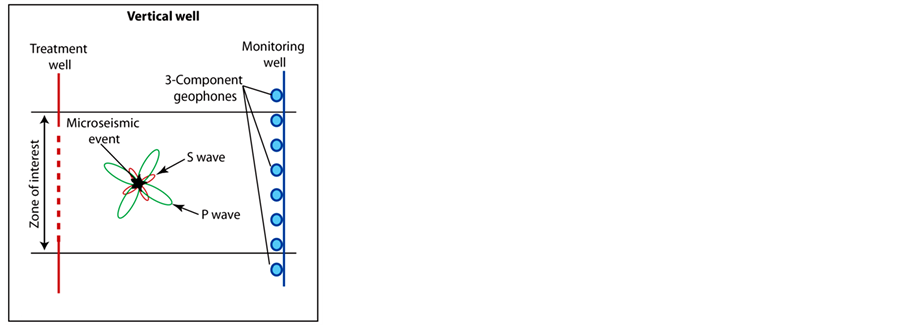
To successfully monitor a hydraulic fracture treatment, the location of the monitoring array, determination of an adequate velocity structure, and management of noise are important issues to be considered [1] . Microseismic imaging usually employs a temporary string of eight to twelve triaxial geophones in a monitoring well located close to the treatment well to observe the creation the of induced fracture systems within its environ (Figure 1).
To capture good quality spectral responses with minimal signal interference in a microseismic record, the downhole geophones should possess sufficient sensor response, minimal tool resonances, and suitable frequency response. In addition, the acquisition system should enable sampling rate between 0.5 and 0.25 msec that corresponds to Nyquist frequency 1000 and 2000 Hz respectively. Seismic attenuation is usually encountered at high frequency signals from far events compared to the low frequency and near ones that are usually mitigated during signal processing. In most cases, microseismic monitoring utilizes downhole sensors, while near surface sensors are in some cases deployed. Being close to the source in borehole microseismic, the depth of the microseismic event is usually accurately determined, but surface arrays proved to be more efficient in determining the spatial location of hypocenter. Dynamic microseismic images are obtained as a live streaming to the fracture propagation using the time history of the microseismic activity [7] . Later, additional seismic source attributes, such as strength or magnitude, are calculated and the complete record is processed to elucidate information about the travel path, e.g. anisotropy and velocity tomograms [8] .
It is well-documented that long-term injection of fluids into deep formations induces earthquakes [9] [10] . This is particularly true in regions susceptible to tectonic activities such as waste chemicals injection in the Rocky Mountains [11] , water injection in geothermal plants [10] [12] , water flooding operation for hydrocarbon production optimization [13] , and water disposal in mining industry [14] . Recently a considerable attention and
 (a)
(a)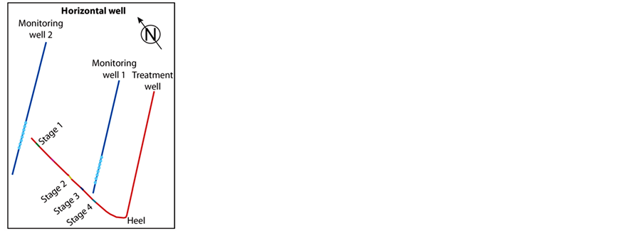 (b)
(b)
Figure 1. Typical microseismic array deployed in vertical well (a) and horizontal well (b).
arguments have been raised concerning the seismicity associating hydraulic fracturing operation [11] , particularly, their role in contaminating the shallow aquifer systems that could be the main water supply for domestic use. Since such operations are not risk-free, several incidents of probable water resources contamination have been reported due to hydrocarbon production stimulation by hydraulic fracking [15] [16] .
Drinking water could be contaminated during hydraulic fracking operations through hidden pathways connecting the producing horizon with shallow aquifer, casing-cement failure, and flowback water used during the treatment. Reference [17] evaluated the potential impacts associating gas-well drilling and fracturing in Marcellus Shale on shallow groundwater systems in northeast Pennsylvania and upstate New York using groundwater analysis. The dissolved-methane concentrations and carbon and hydrogen isotope ratio documented the existence of thermogenic methane in numerous wells with high concentrations (a potential for explosion hazard) close to active natural-gas wells [18] . However, no signs of brine mixture from deeper formations or traces frack treatment fluids were detected. Such observations could be supportive for gas contamination from a near surface origin such as wellbore cement failure, but the deeper origin cannot be entirely excluded due to the extremely low density of methane that enables swift gas to flow across probable hidden pathways, compared to brine and frack treatment fluids. In this paper a detailed discussion on microseismicity associating hydraulic fracking is introduced to assess the potential of hydraulic fracturing to induce minute earthquakes that may jeopardize the surface and near surface environment using microseismic records of different fields, mostly from North America. The results of this research may help recognize the potential/role of hydraulic fracturing of tight petroleum reservoirs in contaminating the potable groundwater aquifers.
2. Methods
Faults are physically static if the in-situ stresses are creating enough frictional forces along fault planes. Fluid injection results in shear stresses within the rock by increasing the pore pressure and therefore weakening the rock fabrics. When the shear stress increases enough to overcome the in-situ stresses, the rock initiates a fracture followed by a slip or directly starts slip on a pre-existing fault plain, resulting in an earthquake.
Reference [19] , approximated the maximum static friction (Fmax static) by:
 (1)
(1)
where:
µstatic is the static friction coefficient; Fnormal is the normal force.
Since microseismic records represent a graphical demonstration to stress decay, fracture geometry and growth behavior can be identified using standard earthquake seismology principles [13] [20] . To evaluate the seismicity associating hydraulic fracturing operation, it is essential to calculate the magnitude for each recorded event and compare the calculated values with injection parameters. Seismic moment can be calculated using source parameters with several techniques, the simplest of them was introduced by reference [21] . He utilized Fourier transform of S-wave displacement to estimate the event moment and radius. In this research, moment and other source parameters data are calculated using Brune’s method.
Reference [21] calculated the Moment (Mо) and the source radius (rо) by
 (2)
(2)
where:
ρ is the density, Vs is the shear velocity, R is the distance from the receivers to the event, Ωo is the low-frequency amplitude of the displacement spectrum, and Fc is a radiation pattern factor. Since the hydraulic fracturing occurs within a small intervals of the producing horizon, the source-receiver distance {R} and radiation pattern factor {Fc} are most likely the influential parameters in Equation (2) to determine the Mo value.
To determine Ωo value for each event, the amplitude spectrum is plotted versus frequency of the microseism after correcting for attenuation. Then the corner frequency is graphically identified by the intersection of the power-law decay at high frequency with the line that approximately represents the low frequency amplitude (Figure 2). The intersection of those two lines indicates the likely corner frequency, which is approximately 350 Hz in the example shown in Figure 2, and the low-frequency amplitude of a little less than 2E−10 m-sec.
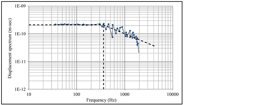
Figure 2. Graphical determination of the corner frequency using amplitude spectrum and frequency after correction for attenuation.
Reference [21] approximated the source radius (ro) as
 (3)
(3)
where:
Kc is a constant, and fc is the corner frequency. The value of the constant Kc has been used to equal (~2.2) by Reference [21] that provides, a conservative value of the size of the slippage plane.
The seismic energy (E) released during the slippage along the fault plane is approximated by Reference [22] as a function of seismic moment by:
 (4)
(4)
Analogous to Richter scale of earthquakes, the moment magnitude (Mw) is a more convenient value to represent seismic moment and/or seismic energy that is obtained by:
 (5)
(5)
where Mo and E in this equation are expressed in dyne-cm.
The slip displacement and area can be determined as a function of the seismic moment by:
 (6)
(6)
where:
μ is the shear modulus of the rock (typically 2.2 × 10⁶ psi for shale), d is the slip distance, and A is the slippage area.
In the present work the calculated moment magnitude from different unconventional reservoirs is subjected to statistical analysis and plotted against various parameters related to the reservoir (e.g. depth) and treatment parameter (e.g. injection rate and volume). This helps understanding the capability of hydraulic fracturing operation to disturb the surface and subsurface environment at the vicinity of stimulated wells.
3. Results and Discussion
3.1. Microseismicity and Treatment Parameters
Thousands of fracturing stimulations have been monitored using a microseismic technique, in which broad variation in the magnitudes of the recorded seismicity is documented. Based on the estimated microseismic magnitudes calculated by Brune’s method [21] described earlier (Equations (2) to (7)), a plot of these values versus depth was constructed for Barnett Shale reservoir (Figure 3, data from Reference [1] ). Although the data points are relatively scattered in this plot, there is a trend of increasing the number of high-magnitude events, shown as dense clusters, with increasing the depth (Figure 3). This reflects the increase of stress in the reservoir rock due to compaction with depth which produces higher strain response in the form of higher microseisms. Another important trend is the linearity of events in either cross-sectional or planar views that could be respectively attributed to numerous small displacements along bedding plains or fault plains. Generally, the majority of microseismic events showed magnitudes less than −0.8 for the shallow zones (less than 2000 m). These values slightly increase to −0.4 with increasing the depth of the target zone (Figure 3 and Figure 4). In few cases microseisms may record Mw values close to 0.5 especially in highly fractured formations such as Barnett Shale (Figure 3) with increasing the depth of the stimulated target. In addition to compaction effect, the variation in magnitudes is influenced by the prevailing geologic structures and/or density of natural fractures that generally controls stress distribution in the stimulated area. Other factors that may influence the variation in magnitude include the treatment parameters such as injection rate, fluid properties, target depth and thickness, completion characteristics, and well design [23] .
The plot of number of events versus magnitude for seismic data typically follows a power law distribution described by the Gutenberg-Richter relationship, (logN = a − bM). However this plot for both Barnett Shale and Cotton Valley reservoirs data set (Figure 4 and Figure 5) had normal distribution patterns for different monitored depth intervals. This could be attributed to inadequate capacity of the recording system to detect smaller magnitudes, Mw < −1.4, at large distance from the monitoring well due to higher signal to noise ratio. In addi-

Figure 3. microseismic magnitudes calculated by Brune’s method plotted versus depth in Barnett shale gas reservoir, Data from Reference [1] .

Figure 4. 994 microseismic events recorded by two monitoring well at depth between 2756 and 2838m in Cotton valley sandstone gas field, East Texas. Data from Reference [24] .
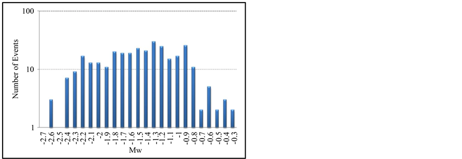
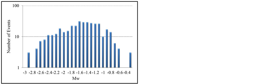
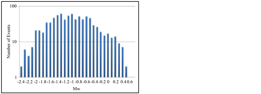
Figure 5. Plot of the number of events versus magnitudes recorded in depth intervals 1170 - 1975 m 1975 - 2200 m and 2200 - 2750 m showed in upper, middle, and lower respectively for the data shown in Figure 3 of Barnett Shale (Data from Reference [1] ).
tion, the high number of events cluster towards the right-hand side (high Mw values, Figure 5 upper part) but the high numbers of recorded events are slightly shifted to the left-hand side of the plot in deeper stimulated intervals (low Mw values, Figure 5 lower part). This shift indicates different magnitudes of completeness (Mc) with deeper monitoring experiments achieving better Mc. Considering a high magnitude event to represent the foot print of initiation of a main fracture or at least activation of some pre-existing ones, the high numbers of strong microseismic events in shallow zones compared to smaller magnitudes reflect the initiation of a major fracture. However, the main fractures in deeper parts propagate for larger distance into the formation since the event magnitudes of the shallow zone are relatively lower than the deep zone and low magnitude (Mw < −1.4) events are distinctly recorded in deeper stimulated intervals (Figure 5).
The injection rate and volume are expected to be influential factors to microseismicity, but could be the most argumentative issues of hydraulic fracking stimulations especially, handling and treatment of the flowback water. To distinguish the relationship between seismicity and both injection rate and injection volume associating hydraulic fracturing stimulations, comprehensive data sets from Barnet shale [1] have been digitized for statistical analysis and interpretation. Figure 6 shows two plots of these data; the first set shows injection rate (m3/minute) versus the recorded moment magnitude and the second displays average magnitude versus the number of the recorded events at the corresponding rate. Although there is a notable increase in the number of recorded events and the average recorded magnitude with increasing the injection rate at the early stages of the treatment (up to 8 m3/minute), such a trend is totally inversed with dramatic changes in rate for the number of events compared to the average recorded magnitude (Figure 6).
The relatively large average magnitudes, reported at injection rate above 10 m3/minute, are attributed to the small number of low magnitude events and the abundant moderate magnitude values. The maximum number of events was recorded at injection rate of 6.0 m3/minute, while the higher average value came slightly later at approximately 8 m3/minute. These observations are common in highly fractured tight formations such as those existing in East Texas, where very small displacements causing small magnitudes are numerous near the treatment well vicinity and remarkably decrease as moving away [25] . Such events are replaced by moderate magnitudes of much lower numbers which are usually arranged parallel to the general structural trends. This may indicate the development of larger stimulated reservoir volume near the treatment well replaced by convey channels away. Furthermore, the relatively larger microseismic magnitudes (Mw > 0) are obviously restricted to the same interval of injection rate which seem critical to this geologic media to create fracture systems. These systems act as effective conduits enough to mitigate the influence of additional increase in injection rate [26] . This may explain the large increase in production rates associating minor seismicity at the first few weeks after treatment (draining the stimulated reservoir volume near the well bore) followed by oscillating pattern that finally collapse to the normal low production rates as clearly shown in Figure 7.
Alternatively, the plot of injection volume versus both number of events and average magnitude values (Figure 8) recorded in two shale reservoirs, Marcellus and Barnett, showed marked increase in seismicity during the first 1600 - 2300 m3 of injected fluids. Through this range, the maximum number of events is recorded after injecting ~1300 m3 of the treatment fluids. Comparing the two plots of Figure 8, the increasing number of events indicates a clear response to the stimulation process at the early stage in which significant displacements along pre-existing fractures and initiation of new fracture systems are expected. After that, the number of events is continually decreasing as a result of the contemporaneous improvement of the local permeability by the fracking process. Such response enhances the local permeability that requires additional volume of treatment fluids and adjustment to injection rate to be able to start new significant seismicity. Despite the clear response of injection volume to seismicity, the average recorded magnitudes were less obvious particularly for Marcellus Shale that shows minute changes through the record (Figure 8). The high average values reported at the later stages is attributed to the significant high proportion of medium-value events compared to the low-value events. It is common for most basins to show similar pattern to that described in Figure 8 with various rates of changes. These results disagree with the conclusion of [1] , who reported the lack of evidence for either rate or volume effects on the size of the microseisms.

Figure 6. Plot of injection rate (m3/minute) versus Moment magnitude recorded during Barnett shale gas stimulation from different fields in East Texas (Data from Reference [1] ).
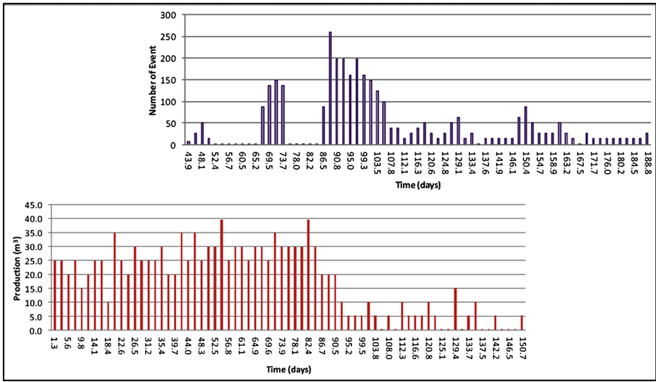
Figure 7. Comparison between production versus time plot and number of events versus time plot for a well in Clinton County, Kentucky. Data from Reference [27] .


Figure 8. Plot of the injected volume of the treatment fluids (m3) versus both number of events and average magnitude recorded during hydraulic fracturing stimulation in Marcellus (upper) and Barnett (lower) shale. Data from Reference [1] .
It is a common practice in hydraulic fracturing operations to begin with a minifrac test and adjust the injection parameters to fit the reservoir condition. Microseismicity usually starts shortly (an hour or so) after the commence of the main treatment (Figure 9). However aseismic events, too small magnitudes to be recorded by downhole tools, most likely exist. On comparing the number of microseismic events to the contemporaneous well head pressure (Figure 9), it is obvious that higher microseismicity is encountered after pressure buildup (between hour 10 and 11), which could have started a little earlier. But as a general pattern, pressure build up with numerous microseismicity is only observed at the early and middle stages of the main treatment (Figure 9). In addition, microseismicity are recorded for few hours after the cease of injection while only few events are encountered during the following weeks of the treatment. In a six months monitoring program by Reference [27] to evaluate the seismicity associating oil production from a tight carbonate reservoir (2% porosity), post a successful hydraulic fracturing job, a total 3200 events of average Mw = −1.2 were recorded during the production of a total of 1250 m3 of oil (Figure 7). The recorded microseismicity during this monitoring program was practically restricted to the stimulated reservoir horizon which indicates a direct relation to recovered-oil production.
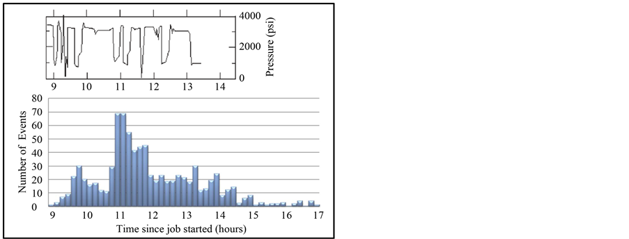
Figure 9. Plot of number of events and Pressure (psi) versus time (hours)since injection started in well CPU2-2, Giddings, Texas. Data from Reference [27] .
A typical seismicity pattern following hydraulic fracturing (Figure 7) shows insignificant microseismic activity in the first 3 months of putting the well on production with a remarkable increase in production rate that usually fluctuates within 30 to 50 % of the total increase in well productivity. By the end of the high production records (90 days period, Figure 7), an unusual increase in seismicity was recorded reflecting abnormal changes taking place within the reservoir followed by continuous decrease in oil production (Figure 7). The recorded seismicity associating diminished well production represents a massive fracture closure or possible fault activation. This may be due to fluid withdrawal from the stimulated reservoir volume that was supporting the overburden pressure and eventually reached failure along the weak zones. There is few recorded seismicity followed these significant modification within the reservoir architecture that extend between days 107 and 170 (Figure 7). This period corresponds to a transition stage towards the stable reservoir condition in which well productivity is dramatically reduced. This pattern represents a typical tight reservoir behavior following hydraulic fracturing stimulations. Such observations indicate a direct relation between the induced seismicity and the efficiency of hydraulic fracking stimulation operations.
The reservoir stimulation efficiency as well as the resulting seismicity varies dramatically among reservoirs and within the same reservoir. However, post-frack high productivity correlates generally with seismicity over wide zones within the producing horizon. Figure 10 shows the cumulative production of two wells that was stimulated by hydraulic fracturing within the same reservoir. In this case the high productivity well showed seismicity over an area 4 - 5 times the stimulated area of the second well. This change in the stimulated reservoir volume is attributed to the reservoir rock competency and durability. Competent rocks favor the development of a single fracture over long distance but durable rocks (highly fractured), prefer fracture propagation over large area rather than long distance [23] [27] . The energy infused into the formation could be dispensed either as numerous micro-fractures or displacement along a fault plane with distinct microseismic record describing each case. Typically, microseismic activity and strength diminishes at the end of the injection treatment and the seismic moment curve stabilizes at approximately minimal values. However, in experiments incorporating fault activation, seismic deformation begins to diminish after the end of injection followed by sharp increase in seismicity that may extend for several tens of minutes before it completely stabilizes. Reference [20] characterized fault activation during hydraulic fracturing of a gas well penetrating a thrust fault. Two different deformation mechanisms: during (fracturing) and after (fault activation) injection were distinctly recognized with two different Frequency-magnitude characteristics. In addition, the P/S amplitude ratio for post injection seismicity are relatively high compared to those recorded during the pumping, suggesting deformation at different orientation that probably include activation of a nearby fault [20] .
3.2. Environmental Repercussions of Hydraulic Fracking
To be felt on land surface, the earthquake’s magnitude should be roughly +3 with approximate energy 2.033 × 10⁹ N-m [1] . This magnitude is too large compared to the magnitude microseism with Mw = −2 and energy 68
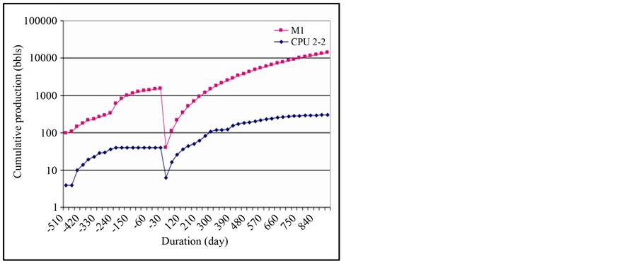
Figure 10. Cumulative production Preand Post-stimulation of two oil wells in Giddings field, Texas. Data from Reference [27] .
N-m. In addition, the detailed discussion of the relation of microseismicity to the depth (Figure 3), magnitude (Figure 4 and Figure 5), injection rate and volume (Figure 6 and Figure 8), and well production (Figure 7 and Figure 10) indicated a conservative framework and limited magnitude of energy. This indicates that the microseismicity associating hydraulic fracking are only located within and/or close to producing horizons that are separated by thousands of rock masses from shallow aquifers. Even microseismicity associating fault activation, within the proximity of a treatment well, may hit nearby deep aquifer [8] . This seems hard to jeopardize near surface groundwater resources unless such faults are naturally good conduits (in such cases fracking only increases contamination that is originally existed). Accordingly, all recorded events do not directly jeopardize the surface environment or the ecology as they cannot be detected except by highly sensitive instruments. Furthermore, hydraulic fracking operation is not expected to induce destructive earthquakes. The USGS inventory of earthquake data since 1900 did not show significant changes compared to the pre-existing data. Therefore, the mechanical hydraulic fracking seems unsuspicious for contaminating the drinking water resources. However, there are substantial hazards entailing the huge volume of treatment fluids that return to the surface charged with chemicals, radioactive materials, and salts. Such fluids are easy to reach nearby rivers and shallow aquifers [28] . In addition, the other possible pathway for gas transport to surface aquifer may take place through the vertical wellbore with poor cement job especially the surface part and/or across the abandoned old well with post fracking cross communication with the producing wells. This indicates the importance and the rising need for better management of shale-gas extraction through integration of the available data, particularly microseismic technology, to improve the industry practices in drilling and hydraulic fracking.
4. Conclusion
The seismicity recorded during hydraulic fracking operations is strongly dependent on the reservoir geology and the parameters of hydraulic treatment. The present study showed that the maximum number of recorded events was recorded at injection rate of 6.0 m3/minute, while the higher average value came slightly later at approximately 8 m3/minute and a marked increase in seismicity is recorded during the first 1600 - 2300 m3 of injected fluids. In addition, the average microseism magnitude (Mw = −2) and energy (68 N-m) presented in this study may indicate limited role of hydraulic fracking stimulations in initiating any destructive earthquakes. This indicates that mechanical processes of hydraulic fracking operations do not directly jeopardize the surface environment or the ecology, but subsurface hazards cannot be totally excluded. The huge volume of treatment fluids that return to the surface charged with chemicals and improper well completion, particularly wellbore cement, represent the important hazardous source. The results of the present study helps understand the behavior of hydrocarbon reservoirs to hydraulic fracking and production operations that may enable a better reservoir management and improve the industry practices in drilling and hydraulic fracking.
Acknowledgements
The author acknowledges very much the authors contributed with the data used in this research and the efforts of their microseismic crews. Also the fruitful suggestions and careful revisions made by Professor Dr. Abdel-Zaher Abouzeid (Professor of Mining Engineering) and Professor Dr. Fouad Khalaf (Professor Petroleum Engineering) at Faculty of Engineering, Cairo University are greatly appreciated.
References
- Warpinski, N.R., Du, J. and Zimmer, U. (2012) Measurements of Hydraulic-Fracture-Induced Seismicity in Gas Shales. SPE Hydraulic Fracturing Technology Conference, Woodlands, 6-8 February 2012, Article ID: 151597.
- Maxwell, S.C., Urbancic, T., Steinsberger, N. and Zinno, R. (2002) Microseismic Imaging of Fracture Complexity in the Barnett Shale. Proceedings, Society of Petroleum Engineers Annual Technical Conference, SPE Annual Technical Conference and Exhibition, San Antonio, 29 September-2 October 2002, Paper # 77440. http://dx.doi.org/10.2118/77440-MS
- Mohammad, N.A. and Miskimins, J.L. (2012) A Comparison of Hydraulic-Fracture Modeling With Downhole and Surface Microseismic Data in a Stacked Fluvial Pay System. SPE Production & Operations Journal, 27, 253-264. http://dx.doi.org/10.2118/134490-PA
- Maxwell, S.C, Du, J. and Shemeta, J. (2008) Monitoring Steam Injection Deformation Using Microseismicity and Tiltmeters. The 42nd U.S. Rock Mechanics Symposium (USRMS), San Francisco, June 29-July 2, 2008, 8.
- Warpinski, N.R., Mayerhofer, M.J., Vincent, M.C., Ceramics, C., Cipolla, C.L. and Lolon, E.P. (2009) Stimulating Unconventional Reservoirs: Maximizing Network Growth While Optimizing Fracture Conductivity. Journal of Canadian Petroleum Technology, 48, 39-51. http://dx.doi.org/10.2118/114173-PA
- Mayerhofer, M.J., Warpinski, N.R., Cipolla, C.L., Walser, D. and Rightmire, C.M. (2010) What Is Stimulated Reservoir Volume? SPE Production & Operations, 25, 89-99. http://dx.doi.org/10.2118/119890-PA
- Ajayi, B., Walker, K., Sink, J., Wutherich, K. and Downie, R. (2011) Using Microseismic Monitoring as a Real Time Completions Diagnostic Tool in Unconventional Reservoirs: Field Case Studies. SPE Eastern Regional Meeting, Columbus, 17-19 August 2011, 10.
- Le Calvez, J.H., Klem, R.C., Bennett, L., Erwemi, A., Craven, M. and Palacio, J.C. (2007) Real-Time Microseismic Monitoring of Hydraulic Fracture Treatment: A Tool To Improve Completion and Reservoir Management. SPE Hydraulic Fracturing Technology Conference, College Station, 29-31 January 2007, 7. http://dx.doi.org/10.2118/106159-MS
- Segall, P. (1989) Earthquakes Triggered by Fluid Extraction. Geology, 17, 942-946. http://dx.doi.org/10.1130/0091-7613(1989)017<0942:ETBFE>2.3.CO;2
- Smith, J.L.B., Beall, J.J. and Stark, M.A. (2000) Induced Seismicity in the SE Geysers Field. Geothermal Resources Council—Transactions, 24, 24-27.
- Nicholson, C. and Wesson, R.L. (1990) Earthquake Hazard Associated with Deep Well Injection—A Report to the U.S. Environmental Protection Agency. U.S. Geological Survey Bulletin 1951. Denver.
- Fehler, M. (1989) Stress Control of Seismicity Patterns Observed during Hydraulic Fracturing Experiments at the Fenton Hill Hot Dry Rock Geothermal Energy Site, New Mexico. International Journal of Rock Mechanics and Mining Sciences & Geomechanics, 26, 211-219. http://dx.doi.org/10.1016/0148-9062(89)91971-2
- Zoback, M.D. and Harjes, H.P. (1997) Injection-Induced Earthquakes and Crustal Stress at 9 km Depth at the KTB Deep Drilling Site, Germany. Journal of Geophysical Research, 102, 18477-18491. http://dx.doi.org/10.1029/96JB02814
- Ake, J., Mahrer, K., O’Connell, D.O. and Block, L. (2005) Deep-Injection and Closely Monitored Induced Seismicity at Paradox Valley, Colorado. Bulletin of the Seismological Society of America, 95, 664-683. http://dx.doi.org/10.1785/0120040072
- Fakete, J. and R. Penty (2011) Environment Canada to Study Hydraulic Fracturing. Post Media News and Calgary Herald. http://www.ernstversusencana.ca/wp-content/uploads/2011/08/2011-09-21-Ottawa-enters-debate-over-shale-gas-development-Environment-Canada-to-study-hydraulic-fracturing.doc
- Chafin, T.D. (1994) Source and Migration Pathways of Natural Gas in Near-Surface Ground Water beneath the Animas River Valley, Colorado and New Mexico. USGS Water Resources Investigations Report 94-4006. http://pubs.er.usgs.gov/usgspubs/wri/wri944006
- S.G. Osborn, Vengosh, A., Warner, N.R. and Jackson, R.B. (2011) Methane Contamination of Drinking Water Accompanying Gas-Well Drilling and Hydraulic Fracturing. Proceedings of the National Academy of Sciences of the United States of America, 108, 8172-8176. http://dx.doi.org/10.1073/pnas.1100682108
- Revesz, K.M., Breen, K.J., Baldassare, A.J. and Burruss, R.C. (2010) Carbon and Hydrogen Isotopic Evidence for the Origin of Combustible Gases in Water Supply Wells in North-Central Pennsylvania. Applied Geochemistry, 25, 1845- 1859. http://dx.doi.org/10.1016/j.apgeochem.2010.09.011
- Tipler, P.A. (1995) Physics for Scientists and Engineers. 3rd Edition, Worth Publishers.
- Maxwell, S.C., Waltman, C.K., Warpinski, N.R., Mayerhofer, M.J. and Boroumand, N. (2009) Imaging Seismic Deformation Induced by Hydraulic Fracture Complexity. SPE Reservoir Evaluation & Engineering Journal, 12, 48-52. http://dx.doi.org/10.2118/102801-PA
- Brune, J.N. (1970) Tectonic Stress and the Spectra of Seismic Shear Waves from Earthquakes. Journal of Geophysical Research, 75, 4997-5009. http://dx.doi.org/10.1029/JB075i026p04997
- Kanamori, H. (1977) The Energy Release in Great Earthquakes. Journal of Geophysical Research, 82, 2981-2987. http://dx.doi.org/10.1029/JB082i020p02981
- King, G.E. (2010) Thirty Years of Gas Shale Fracturing: What Have We Learned? SPE Annual Technical Conference and Exhibition held in Florence, Italy, 19-22 September 2010, 50.
- Urbancic, T.I., Shumila, V., Rudledge, J.T. and Zinno, R.J. (1999) Determining Hydraulic Fracture Behavior Using Microseismicity. The 37th U.S. Symposium on Rock Mechanics (USRMS), Vail, 7-9 June 1999, 8.
- Abdulaziz, M. (2013) Microseismic Imaging of Hydraulically Induced-Fractures in Gas Reservoirs: A Case Study in Barnett Shale Gas Reservoir, Texas, USA. OJG, 3, 361-369.
- King, G.E. (2012) Hydraulic Fracturing 101: What Every Representative, Environmentalist, Regulator, Reporter, Investor, University Researcher, Neighbor and Engineer Should Know About Estimating Frac Risk and Improving Frac Performance in Unconventional Gas and Oil Wells. SPE Hydraulic Fracturing Technology Conference, Woodlands, 6-8 February 2012, 80.
- Phillips, W.S., Rutledge, J.T., Fairbanks, T.D., Gardner, T.L., Miller, M.E. and Schuessler, B.K. (1998) Reservoir Fracture Mapping using Microearthquakes: Austin Chalk, Giddings Field, TX and 76 Field, Clinton Co., KY. SPE Reservoir Evaluation & Engineering Journal, 1, 114-121. http://dx.doi.org/10.2118/36651-PA
- Mooney, C. (2011) The Truth about Fracking. Scientific American Magazine, November 2011. http://www.scientificamerican.com/article.cfm?id=the-truth-about-fracking