Open Journal of Earthquake Research
Vol.2 No.2(2013), Article ID:31299,5 pages DOI:10.4236/ojer.2013.22003
On the Relative Effect of Magnitude and Depth of Earthquakes in the Generation of Seismo-Ionospheric Perturbations at Middle Latitudes as Based on the Analysis of Subionospheric Propagation Data of JJY (40 kHz)-Kamchatka Path
1Advanced Wireless Communications Research Center, University of Electro-Communications (UEC), Tokyo, Japan
2Hayakawa Institute of Seismo Electromagnetics, Co. Ltd., UEC Incubation Centre, Tokyo, Japan
3Institute of Physics of the Earth, Russian Academy of Sciences, Moscow, Russia
Email: hayakawa@hi-seismo-em.jp, rozhnoi@ifz.ru
Copyright © 2013 Masashi Hayakaw et al. This is an open access article distributed under the Creative Commons Attribution License, which permits unrestricted use, distribution, and reproduction in any medium, provided the original work is properly cited.
Received March 6, 2013; revised April 12, 2013; accepted May 7, 2013
Keywords: VLF/LF Subionospheric Propagation; Ionospheric Perturbation; Earthquake precursors; Earthquake Prediction
ABSTRACT
The relative importance of magnitude and depth of an earthquake (EQ) in the generation of seismo-ionospheric perturbations at middle latitudes is investigated by using the EQs near the propagation path from the Japanese LF transmitter, JJY (at Fukushima) to a receiving station at Petropavsk-Kamchatsky (PTK) in Russia during a three-year period of 2005-2007. It is then found that the depth (down to 100 km) is an extremely unimportant factor as compared with the magnitude in inducing seismo-ionospheric perturbations at middle latitudes. This result for sea EQs in the Izu-Bonin and Kurile-Kamchatka arcs is found to be in sharp contrast with our previous result for Japanese EQs mainly of the fault-type. We try to interpret this difference in the context of the lithosphere-atmosphere-ionosphere coupling mechanism.
1. Introduction
There have been found different kinds of electromagnetic precursors of earthquakes (EQs), and the presence of those seismo-electromagnetic precursors is recently considered to be an irrefutable fact, though the physics of these phenomena remains poorly understood. (e.g., Molchanov and Hayakawa (2008) [1], Hayakawa (Ed.) (2009, 2012) [2,3], Uyeda et al. (2009) [4], and Hayakawa and Hobara (2010) [5]). Such electromagnetic EQ precursors can be customarily classified into the two types. The first type is the direct effects such as electromagnetic radiation from the lithosphere in a wide frequency range, while the second is the indirect effect such as seismoatmospheric and ionospheric perturbations as detected by means of propagation anomalies of transmitter signals in different frequency ranges. When utilizing any one of those precursors for the practical short-term EQ prediction, the most important issue is whether the precursor is statistically correlated with EQs or not, which can be only possible by analyzing a huge number of events based on the long-term observation.
Among many EQ precursors [1-5], the most promising one from the statistical point of view is the ionospheric perturbation, because the perturbations both in the lower ionosphere and upper ionosphere (F region) are found to be statistically significantly correlated with EQs. Hayakawa et al. (2010) [6,7] have obtained the significant statistical correlation between subionospheric VLF/LF propagation anomalies and EQs as for the lower ionospheric perturbation. On the other hand, Liu (2009) [8] has presented the result on the statistical correlation of the foF2 in the upper ionosphere with EQs. This paper deals with the lower ionospheric perturbations detected by subionospheric VLF/LF propagation anomalies. Hayakawa et al. (2010) [6] have found that a significant correlation is established for an EQ with significant magnitude (M) ˃ 5.5 [9,10] and shallow depth (D) (D less than 40 - 50 km). These results are based on the observation in and around Japan (that is, mainly inland (or fault-type) EQs). So that, the influence of D is rather evident in generating seismo-ionospheric perturbations for EQs in Japan.
We would like to explore whether this conclusion is still valid for EQs in other geological areas or at different latitudes. By using the VLF/LF subionospheric propagation data from the JJY (Fukushima, Japan) to Petropavlovsk-Kamchatsky (PTK), Russia, we will study, in this paper, the relative importance of M and D of an EQ in generating seismo-ionospheric disturbances over this midlatitude propagation path in order to explore whether there exists a significant difference in the characteristics of seismo-ionospheric perturbations of Japanese EQs and sea EQs. Finally, we discuss this difference in the context of the lithosphere-ionosphere coupling mechanism.
2. EQs and LF Propagation Data
In order to study the relative importance of M and D of an EQ in generating the seismo-ionospheric perturbation at middle latitudes, we will analyze the dependence of amplitude of the LF signal. For the analysis, we use the LF signal recorded at Petropavlovsk-Kamchatsky (PTK) station (geographic coordinates; 53˚09'N, 158˚55'E) in Russia from a Japanese transmitter with call sign of JJY (40 kHz) located at Fukushima [11]. The positions of the transmitter and receiving stations are illustrated in Figure 1 and the distance between the transmitter and receiver is 2300 km. The data from three years (2005, 2006 and 2007) are used.
As a main characteristic of the LF signal, we estimate the difference between the current nighttime amplitude
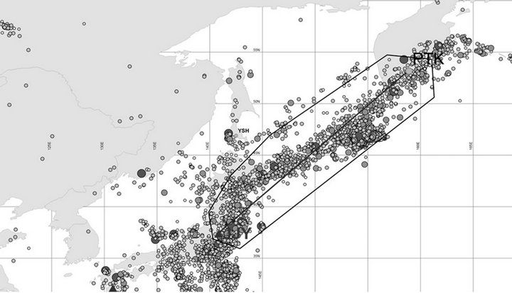
Figure 1. Relative location of the LF observing station in Petropavlovsk-Kamchatsky (PTK) in Russia, the LF transmitter JJY (40 kHz) in Fukushima, and epicenters of EQs with M ˃ 4 (catalogue of USGS) for three years of 2005- 2007. The area around the wave path of JJY-PTK is encircled by a black line.
and the monthly averaged amplitude calculated over night (this is called the conventional nighttime fluctuation method [11,10,6,7]).
The epicenters of EQs with M ≥ 4 from the catalogue of USGS (United States Geological Survey) are shown in Figure 1. We select the EQs with D less than 100 km and with epicenters close to the great-circle path between the transmitter and the receiver. One circle indicates an EQ, with its size reflecting the EQ M. As seen from this plot, many EQs are found to be located in the offsea of Hokkaido, Kurile islands and Kamchatka. At first we select the area around the wave path of JJY-PTK (like wave sensitive Fresnel zone), which is indicated by a black line in addition to the great-circle path of JJY-PTK in Figure 1. Then for every EQs in this area we calculate the radius of a zone for which the ionospheric precursor of an EQ may be found. According to Dobrovsky et al. (1979) [12], the preparation radius is given by R = 100.43 M. We also compute the distance (L) from the EQ epicenter to the great-circle path. In the following analysis we have included only EQs satisfying tentatively the ratio R/L ≥ 0.7. When we have several EQs on one particular day, we have selected the largest M EQ.
Figure 2 illustrates the distributions of EQs as a function of EQ M. The upper panel represents the total number of EQs on the basis of selection depending on D and distance from the great-circle path (R/L ≥ 0.7). The bottom panel illustrates the number of EQs after the further selection of the largest M on one day. In the latter case (bottom panel in Figure 2), the number of EQs with 4.5 ≤ M ≤ 5.5 is, on the contrary, more than that of EQs with 4.0 ≤ M ≤ 4.5. After this selection the total number of EQs is 543.
3. Analysis Results
Rozhnoi et al. (2004) [11] analyzed the data from the same propagation path of JJY-PTK during two years of
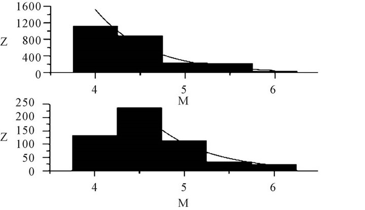
Figure 2. Distributions of EQs as a function of M. Upper panel shows the total number of EQs selected based on the D and the distance from the great-circle path (R/L ≥ 0.7) and bottom panel shows the number of EQs after the selection of the largest M in a day. Black curve is a regression curve.
2001 and 2002. Then, in addition to the analyses of solar and geomagnetic effects in subionospheric LF data, they came to the conclusion that the seismic effect on this LF signal is observed only for EQs with M ≥ 5.5 and the anomaly appears a few to several days before an EQ. Figure 3 illustrates the results of our analysis. The analysis was performed for a day when an EQ occurred (Day-0 in Figure 3) and during 5 days before the EQ (Day-1 to Day-5 in Figure 3). The ordinate (y axis) represents the amplitude of the LF signal averaged over night and normalized by the standard deviation (σ). While, the abscissa (x axis) is M/D (M: magnitude in Richter scale and D in km). If we would expect the similar effect of EQ D as in the results for Japanese EQs [6,7], we would anticipate that the signal amplitude would exhibit a significant increase with M/D. However, the correlation coefficients between the normalized amplitude and M/D in all plots in Figure 3, are found to be very weak of the order of 0.1, which means nearly no correlation between LF signal amplitude and M/D. So that, the regression equation for each scatter plot is not so meaningful. This means that the EQ D seems to be not so important as compared with M in inducing the seismoionospheric perturbation at middle latitudes in this paper. In any case, two groups of dots are seen in all plots of Figure 3, which corresponds to different Ds in the subduction area of our interest. One group includes EQs with 0 ≤ D ≤ 20 km, and another group of dots includes EQs with 20 < D < 100 km. The area of sensitivity along the wave path in Figure 1 is seen to cover highly seismically active Izu-Bonin and Kurile-Kamchatka arcs. The epicentral zone can be divided into the different regions which are characterized by distinctly different seismic activity and focal zone depths. Maximal focal depths in this region are 600 - 650 km, and the upper mantle has a complicated mosaic-layered structure [11], composed of two characteristic layers as in Figure 3. The distributions of EQs depending on EQ M for two groups are shown in Figure 4. In the left the distribution of EQ M is observed for the first group of dots (deep EQs), in which we notice a nearly uniform temporal variation over the three years, with a large EQ on November 15, 2006. In the right panel of Figure 4 we find that the temporal evolution of shallow EQs is very inhomogeneous over three years and that the period with increasing the number of EQs (shallow EQ, 0 < D < 20 km) is clearly observed during October 2006 to June 2007.
4. Concluding Remarks and Discussion
Based on the data analysis for three years (2005-2007) for the propagation path of JJY-PTK, we have investigated the relative importance of M and D in generating the seismo-ionospheric perturbations for sea EQs in the Kurile-Kamchatka region. Then we come to the follow
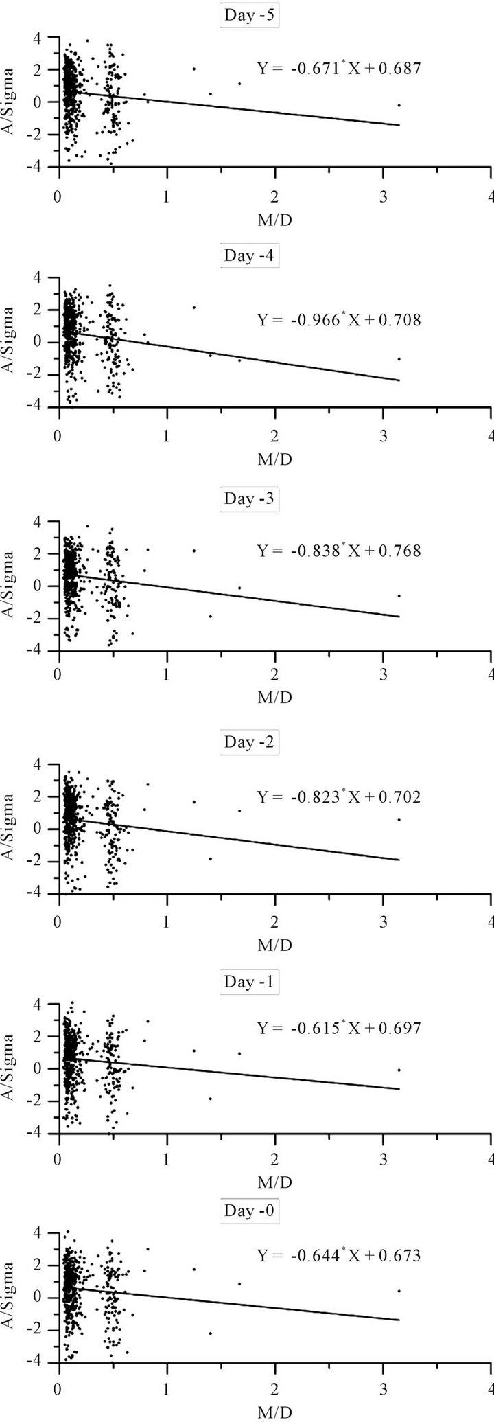
Figure 3. Dependences of amplitude of the LF signal on the parameter of M/D 1 - 5 days before an EQ (Day-1 - 5) and on the day of the EQ (Day-0). The ordinate is the LF signal intensity normalized by the standard deviation (σ).
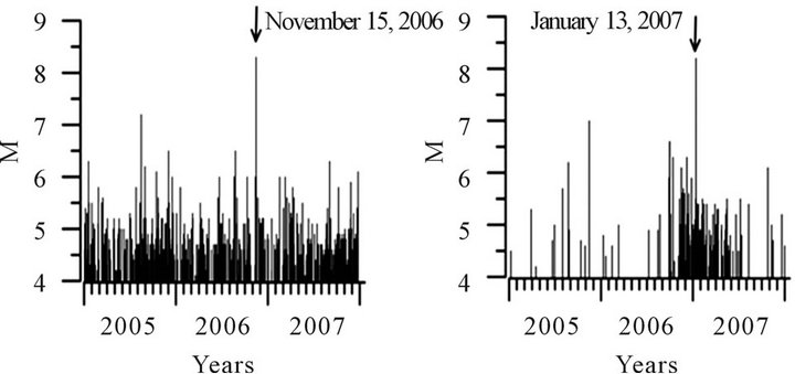
Figure 4. Temporal distributions of EQs as a function of M for two groups of dots. The left is for D larger than 20 km (deep EQs), and the right is for D smaller than 20 km (shallow EQs).
ing conclusion.
1) We have analyzed over 400 EQ events in order to study the correlation of LF signal intensity with a new parameter of M/D.
2) During several days before an EQ and on the day of the EQ, the LF signal intensity is found to exhibit nearly no correlation with M/D.
3) The above result is indicative that the EQ D is not so important as EQ M in the generation of seismo-ionospheric perturbations. Namely, EQ M is of the major importance in generating seismo-ionospheric perturbations at middle latitudes. This is the conclusion in the area of JJY-PTK path and for EQs with D less than 100 km.
The above result for sea EQs in the Kurile-Kamchatka region appears to be in sharp contrast with our previous statistical results for Japanese inland EQs. Hayakawa et al. (2010) [6] have analyzed the EQs mainly taken place inland; that is, their target EQs are of the fault-type, and they have found a significant effect of D. Namely, ionospheric perturbations are excited only by shallow (D ~40 - 50 km) EQs (with M ≥ 6.0), but it is difficult for us to find the ionospheric perturbation for deep (D ˃ 50 km) EQs (with M ≥ 6.0). This point is consistent with a recent Japanese work by Kon et al. (2011) [13]. Of course, it may be possible that a very large (M ˃ 7) EQ can induce the seismo-ionospheric perturbation even for D of the order of ~100 km.
When discussing the characteristics of VLF/LF perturbations at middle latitudes in this paper and in our previous paper [6], the first point for a possible difference is the latitudinal effect. Because Kamchatka is located at middle geomagnetic latitudes much higher than our Japanese low-latitudes [6,9], a majority of subionospheric VLF/LF perturbations are caused by solar-terrestrial effects such as solar flares, geomagnetic activities and only ~30% of the perturbations are related with EQs with M ≥ 5.5 [11]. On the other hand, the influence of solar-terrestrial effects on subionospheric VLF/LF propagation anomalies (though it does exist) is drastically smaller at low latitudes such as Japan, and the “local” subionospheric VLF/LF propagation in Japan is highly likely to be related with EQs.
The clear discrepancy of the properties of seismoionospheric perturbation for inland and sea EQs is likely to be an important finding to be discussed in the context of lithosphere-atmosphere-ionosphere (LAI) coupling mechanism. There has been published a recent statistical study by Parrot (2012) [14], who has statistically studied the seismo-ionospheric perturbation (in the upper ionosphere) based on the about 5 years observation by the DEMETER satellite. His most fundamental point is that the ionospheric perturbation increases with increasing the EQ M. The second point is that more intense perturbation is observed for sea EQs than inland EQs; in other words, perturbations are not so important for deep (D ˃ 40 km) EQs. In the conjunction with these statistical results by Parrot (2012) [14] we will try to reconsider our results in this paper. In the analysis of this paper dealing with EQs in the offshore of Hokkaido, Kurile Islands and Kamchatka, these EQs take place in the subduction region of Pacific plate, and these are believed to belong to sea EQs. Stronger perturbation is expected for sea EQs as shown in Parrot (2012) [14], which seems to be consistent with the insignificant effect of D (only down to 100 km) in our seismo-ionospheric perturbation for sea EQs in this paper. It is definite from our previous studies [9,11] and Parrot’s result that the EQ M is the most essential parameter for seismo-ionospheric perturbations at any latitudes. It is easy for us to understand that the fact by Hayakawa et al. (2010) [6] that mainly shallow (D < 40 km) EQs are able to induce the ionospheric perturbation, seems to be consistent with Parrot (2012) [14] result which has indicated a small perturbation for inland EQs than for sea EQs.
There have been proposed two major hypotheses of LAI coupling; 1) electric field channel [15,16] and 2) atmospheric oscillation channel [e.g., 1,17,18]. In the model by Pulinets (2009) [15] radioactive radon is the main player, while Freund (2009) [16] assumes the appearance of positive holes. As for the second hypothesis, we have presented a lot of observational evidences in support to this channel [19] though there are very few observational results on the precursory physical processes near the ground surface [20]. Here we attempt to use the sea/land EQ asymmetry in the study of generation of seismo-ionospheric perturbation in order to elucidate which mechanism is more plausible.
In the case of second hypothesis, we have to take a fundamental premise that there must be present some kind of fluctuations on or near the ground surface (either ground motion, or any changes in atmospheric pressure (or temperature) or so). How to interpret the sea/land EQ asymmetry (stronger perturbation for sea EQs) in this hypothesis? For sea EQs, we assume ground motions in the sea bed, which might lead to the sea surface waves with small amplitude but horizontally extended. This might form a great piston that pushes and pulls the air above the EQ hypocenter, which means that the sea surface is a good plough for exciting the atmospheric gravity waves and then leading to seismo-ionospheric perturbations. While, the ground EQ is considered to be a poor plough in the sense of launching the atmospheric gravity waves. On the other hand, when thinking of the 1st channel, there exists a difficulty to account for how to generate stronger electric field for the sea EQs. One point by Parrot (2012) [14] as related to the land/sea EQ asymmetry is that the electric conductivity above the sea due to the less contaminated condition than on the ground (land), which might be related with the 1st hypothesis. However it is not clear how this land/sea EQ asymmetry can be explained by electric field mechanisms.
REFERENCES
- O. A. Molchanov and M. Hayakawa, “Seismo Electromagnetics and Related Phenomena: History and Latest results,” TERRAPUB, Tokyo, 2008, 189 p.
- M. Hayakawa, “Electromagnetic Phenomena Associated with Earthquakes,” Transworld Research Network, Trivandrum, 2009, 279 p.
- M. Hayakawa, “The Frontier of Earthquake Prediction Studies,” Nihon-Senmontosho-Shuppan, Tokyo, 2012, 794 p.
- S. Uyeda, T. Nagao and M. Kamogawa, “Short-Term Earthquake Prediction: Current State of Seismo-Electromagnetics,” Tectonophysics, Vol. 470, No. 3-4, 2009, pp. 205-213. doi:10.1016/j.tecto.2008.07.019
- M. Hayakawa and Y. Hobara, “Current Status of SeismoElectromagnetics for Short-Term Earthquake Prediction,” Geomatics, Natural Hazards and Risk, Vol. 1, No. 2, 2010, pp. 115-155. doi:10.1080/19475705.2010.486933
- M. Hayakawa, Y. Kasahara, T. Nakamura, F. Muto, T. Horie, S. Maekawa, Y. Hobara, A. A., Rozhnoi, M. Solivieva and O. A. Molchanov, “A Statistical Study on the Correlation between Lower Ionospheric Perturbations as Seen by Subionospheric VLF/LF Propagation and Earthquakes,” Journal of Geophysical Research: Space Physics, Vol. 115, No. A9, 2010, Article ID: A09305. doi:10.1029/2009JA015143
- M. Hayakawa, Y. Kasahara, T. Nakamura, Y. Hobara, A. Rozhnoi, M. Solovieva and O. A. Molchanov, “On the Correlation between Ionospheric Perturbations as Detected by Subionospheric VLF/LF Signals and Earthquakes as Characterized by Seismic Intensity,” Journal of Atmospheric and Solar-Terrestrial Physics, Vol. 72, No. 13, 2010, pp. 982-987. doi:10.1016/j.jastp.2010.05.009
- J. Y. Liu, “Earthquake Precursors Observed in the Ionospheric F-Region,” In: M. Hayakawa, Ed., Electromagnetic Phenomena Associated with Earthquakes, Transworld Research Network, Trivandrum, 2009, pp. 187-204.
- S. Maekawa, T. Horie, T. Yamauchi, T. Sawaya, M. Ishikawa, M. Hayakawa and H. Sasaki, “A Statistical Study on the Effect of Earthquakes on the Ionosphere, Based on the Subionospheric LF Propagation Data in Japan,” Annales Geophysicae, Vol. 24, 2006, pp. 2219- 2225. doi:10.5194/angeo-24-2219-2006
- Y. Kasahara, F. Muto, T. Horie, M. Yoshida, M. Hayakawa, K. Ohta, A. Rozhnoi, M. Solovieva and O. A. Molchanov, “On the Statistical Correlation between the Ionospheric Perturbations as Detected by Subionospheric VLF/LF Propagation Anomalies and Earthquakes,” Natural Hazards and Earth System Sciences, Vol. 8, 2008, pp. 653-656. doi:10.5194/nhess-8-653-2008
- A. Rozhnoi, M. S. Solovieva, O. A. Molchanov and M. Hayakawa, “Middle Latitude LF (40 kHz) Phase Variations Associated with Earthquakes for Quiet and Disturbed Geomagnetic Conditions,” Physics and Chemistry of the Earth, Vol. 29, No. 4-9, 2004, pp. 589-598. doi:10.1016/j.pce.2003.08.061
- J. R. Dobrovolsky, S. I. Zubkov and V. I. Myachkin, “Estimation of the Size of Earthquake Propagation Zones,” Pure and Applied Geophysics, Vol. 117, No. 5, 1979, pp. 1025-1044. doi:10.1007/BF00876083
- S. Kon, M. Nishihashi and K. Hattori, “Ionospheric Anomalies Possibly Associated with M ≥ 6.0 Earthquakes in the Japan Area during 1998-2010: Case Studies and Statistical Study,” Journal of Asian Earth Science, Vol. 41, 2011, pp. 410-420.
- M. Parrot, “Statistical Analysis of Automatically Detected Ion Density Variations Recorded by DEMETER and Their Relation to Seismic Activity,” Annales Geophysicae, Vol. 55, 2012, pp. 149-155.
- S. Pulinets, “Lithosphere-Atmosphere-Ionosphere Coupling (LAIC) Model,” In: M. Hayakawa, Ed., Electromagnetic Phenomena Associated with Earthquakes, Transworld Research Network, Trivandrum, 2009, pp. 235-253.
- F. Freund, “Stress-Activated Positive Hole Change Carriers in Rocks and the Generation of Pre-Earthquake Signals,” In: M. Hayakawa, Ed., Electromagnetic Phenomena Associated with Earthquakes, Transworld Research Network, Trivandrum, 2009, pp. 41-96.
- O. A. Molchanov, “Lithosphere-Atmosphere-Ionosphere Coupling Due to Seismicity,” In: M. Hayakawa, Ed., Electromagnetic Phenomena Associated with Earthquakes, Transworld Research Network, Trivandrum, 2009, pp. 255-279.
- V. Korepanov, M. Hayakawa, Y. Yampolski and G. Lizunov, “AGW as a Seismo-Ionospheric Coupling Responsible Agent,” In: M. Hayakawa, J. Y. Liu, K. Hattori and L. Telesca, Eds., Electromagnetic Phenomena Associated with Earthquakes and Volcanoes, 2009, pp. 485-495.
- M. Hayakawa, Y. Kasahara, T. Nakamura, Y. Hobara, A. Rozhnoi, M. Solovieva, O. A. Molchanov and V. Korepanov, “Atmospheric Gravity Waves as a Possible Candidate for Seismo-Ionospheric Perturbations,” Journal of Atmospheric Electricity, Vol. 31, No. 2, 2011, pp. 129-140.
- C. H. Chen, T. K. Yeh, J. Y. Liu, C. H. Wang, S. Wen, H. Y. Yen and S. H. Chang, “Surface Deformation and Seismic Rebound: Implications and Applications,” Surveys in Geophysics, Vol. 32, No. 3, 2011, pp. 291-313. doi:10.1007/s10712-011-9117-3