Open Journal of Earthquake Research
Vol. 2 No. 1 (2013) , Article ID: 28378 , 20 pages DOI:10.4236/ojer.2013.21001
A Wavelet Transform Method to Detect P and S-Phases in Three Component Seismic Data
1Earthquake Monitoring Center, Sultan Qaboos University, Muscat, Oman
2University of Newcastle upon Tyne, Newcastle upon Tyne, UK
3Institute of Geophysics and Planetary Physics, University of California, San Diego, USA
Email: *salam95@squ.edu.om
Received December 6, 2012; revised January 14, 2013; accepted 5 February 2013
Keywords: Discrete Time Wavelet Transform; P and S-phases; Automatic Detection; Rectilinearity Function
ABSTRACT
The discrete time wavelet transform has been used to develop software that detects seismic P and S-phases. The detection algorithm is based on the enhanced amplitude and polarization information provided by the wavelet transform coefficients of the raw seismic data. The algorithm detects phases, determines arrival times and indicates the seismic event direction from three component seismic data that represents the ground displacement in three orthogonal directions. The essential concept is that strong features of the seismic signal are present in the wavelet coefficients across several scales of time and direction. The P-phase is detected by generating a function using polarization information while S-phase is detected by generating a function based on the transverse to radial amplitude ratio. These functions are shown to be very effective metrics in detecting P and S-phases and for determining their arrival times for low signal-to-noise arrivals. Results are compared with arrival times obtained by a human analyst as well as with a standard STA/LTA algorithm from local and regional earthquakes and found to be consistent.
1. Introduction
Seismic events such as earthquakes cause a release of energy represented by seismic waves that can be recorded by seismic monitoring stations. Detection of seismic waves and estimation of their arrival times provides information about earthquake location and magnitude. Analysis and detection of seismic waves may be done by visual inspection by a trained analyst or automatic analysis software.
Rapid and accurate detection of seismic waves is of great importance in locating earthquakes [1-10]. Automatic detection techniques are of interest because they can be processed in near real-time; they apply a consistent set of metrics and are repeatable. However, it is often very difficult to determine consistent estimates of P and S waves if they have low signal-to-noise characteristics, particularly if arriving at seismic stations at regional distances.
The objectives of this research are:
1) To design an algorithm for the detection and analysis of the two main types of seismic body waves (P and S-phases).
2) To test the algorithm using seismic events recorded by various stations at local and regional distances, and then compares the results with the results obtained by other methods.
Several methods have been tried recently these that have involved digital signal processing in both time and frequency domains [11-13]. The method adopted here is wavelet transform using an approach initially developed by K. Anant and F. Dowla [11].
The algorithms have been developed in Matlab 6.5TM (http://www.mathworks.com) including signal processing and WaveLabTM (http://www-stat.stanford.edu/~wavelab) toolboxes. WaveLab is a library of Matlab routines for wavelet analysis, wavelet-packet analysis, cosine-packet analysis and matching practice. The algorithms can be run on a laptop with 256 MB RAM or on a mainframe computer.
Seismic Data Used in Testing
Seismic data from Earthquake Monitoring Center in Oman has been used for testing the algorithms. The ANZA Broadband Seismic Network (http://eqinfo.ucsd.edu) also provided analyst reviewed data and STA/LTA automatic detected data used for comparison with the wavelet detector.
The paper structured as follows: An introduction about wavelet transform is given in Section 2. Section 2 also includes description of the discrete time wavelet transforms, its application on seismic signals to match specific features and how the selection of wavelet type has been done in this study. The multiresolution analysis technique and the perfect reconstruction filter banks are explained too. The developed software and methodology are explained in Section 3. The flow charts of the algorithms are illustrated in Appendix B and a detailed annotation is given in Section 3 too. The results are discussed in Section 4. Comments about the testing results and the comparison results with other methods are presented in Section 5.
2. Wavelet Transform Analysis
2.1. Introduction
The wavelet transform is a very useful tool for analysing noisy and transient signals and has the ability to represent the signal in both its time and frequency domains. It is a very useful tool in the analysis of non-stationary signals such as seismic signals due to its ability to resolve features at various scales [14].
The wavelet theory arises in 1909 when Haar constructs the first orthonormal system of compactly supported functions called the Haar basis [15].
The term wavelet has been coined in the field of seismology in 1940 by Ricker, N. [15]. The wavelet theory has been applied on seismic signals by Grossmann and Morlet in 1984 [11]. In 1988, Daubechies developed an orthonormal, compactly supported wavelet basis that is smoother than Haar basis [14-16]. Application of wavelet transform on seismic signals has been done by Anant and Dowla [11], Oonincx, P. J. [12] as well as by Zhang et al. 2003 [13].
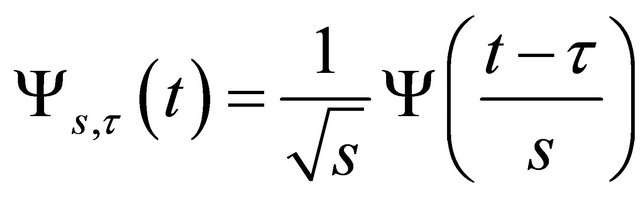
The wavelets form a family. The basic form is called the mother wavelet. All the daughter wavelets are derived from this wavelet according the following equation:
 (2.1)
(2.1)
where, s and  are the scale and translation of the daughter wavelet. The term s−1/2 normalizes the energy for different scales, whereas the other terms define the width and translation of the wavelet.
Digital signal analysis using wavelet transforms begins with the construction of a single parent wavelet. The signal is then decomposed into a series of basis functions of finite length consisting of dilated (stretched) and translated (shifted) versions of this parent wavelet function, i.e., wavelets of different scales and positions in time or space. This process is similar to Fourier analysis, where the parent wavelet is analogous to the sine wave, and the basis functions in Fourier decomposition are sine waves of various amplitude, phase, and frequency variations of the parent sine wave [14,17].
Scaling a wavelet simply means stretching (or compressing) it. The smaller the scale factor, the more “compressed” the wavelet. The more stretched the wavelet, the longer the portion of the signal with which it is being compared, and thus the coarser the signal features being measured by the wavelet coefficients. Thus, there is a correspondence between wavelet scales and frequency as revealed by wavelet analysis:
• Low scale s  compressed wavelet
  rapidly changing details
  High frequency ω.
• High scale s  Stretched wavelet
  Slowly changing, coarse features
  Low frequency ω.
The decomposition advantage is very useful in dealing with signals contain features with various frequency characteristics. Another advantage of the wavelet transform is that its analysis can be chosen based on the application [11].
Figure 1 shows seismic signal at top and wavelet coefficients of six scales where “Daubechies 8” wavelet has been used. The smallest scale is the one that contains the highest frequency while the largest scale is the one that contain the lowest frequency.
2.2. The Discrete Time Wavelet Transform
A discrete type of wavelet transform exists, termed the discrete time wavelet transform (DTWT), where scales and shifts take on discrete values. It allows fast computation of the transform for the digitized signals and gives perfect signal reconstruction. It is a form of multiresolution analysis and is related to perfect reconstruction filter banks [14,18,19].
The wavelet transform can be applied to seismic signals in terms of the type of decomposition as well as in terms of pattern matching [11,12].
In wavelet analysis, we often speak of approximations and details. The approximations are the high-scale, lowfrequency components of the signal while the details are the low-scale, high-frequency components. Figure 2 shows that the input signal is filtered by a low-pass and high-pass filters in one stage wavelet transform. Then, the signal is down-sampled by a factor of 2 to produce DWT coefficients.
2.2.1. Subband Coding
The DTWT is implemented using the sub-band coding scheme represented in Figure 3" target="_self"> Figure 3. The signal is decomposed into 2 frequency bands: low (approximations) and high (details). For the approximation and detail coefficients to represent a discrete-time wavelet decomposition H and G filters must belong to a perfect reconstruction filter bank and required to be regular [14,18,20,21].
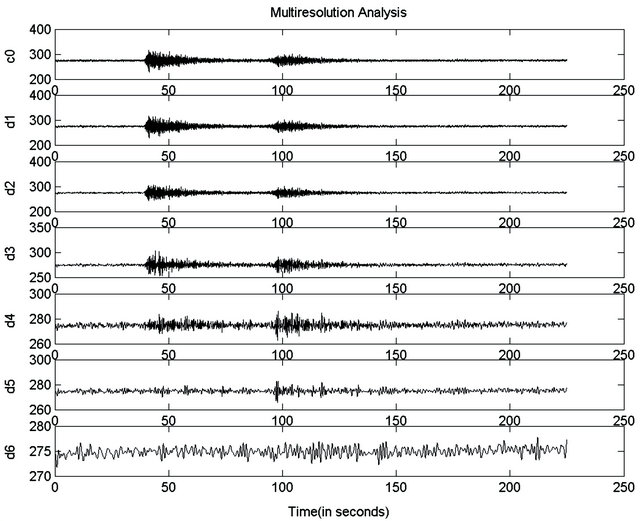
Figure 1. Seismic signal decomposed into several scales.
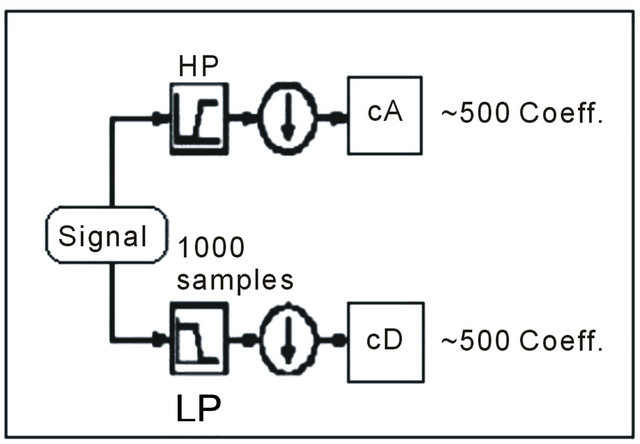
Figure 2. One stage wavelet transforms.
The wavelet analysis involves filtering and downsampling while the wavelet reconstruction process consists of up-sampling and filtering. Up-sampling is increasing the number of samples by inserting zeros between samples.
The following filters then perform an interpolation by filling in the zero points with the appropriate signal information.
The filtering part of the reconstruction process bears some discussion, because it is the choice of filters that is crucial in achieving perfect reconstruction of the original signal.
Figure 4 is a typical example of such filters magnitude responses.
The down-sampling of the signal components performed during the decomposition phase introduces a distortion called aliasing. It turns out that by carefully choosing filters for the decomposition and reconstruction phases that are closely related, we can “cancel out” the effects of aliasing.
In order for the lowand high-pass decomposition filters (H and G), together with their associated reconstruction filters (L* and G*) shown in Figure 3 to perform such decomposition and reconstruction a system of what is called Quadrature Mirror Filters is used [14,17,19].
2.2.2. Quadrature Mirror Filters
QMF banks are a set of finite impulse response (FIR) filters that enable a signal to be decomposed into subbands and allow reconstruction of the signal from the sub-bands without distortion. It is an example of decimation and interpolation and allows designing two-channel perfect reconstruction filter banks and therefore to generate wavelet bases.
The analysis filters have typically low pass and high pass frequency responses with a cutoff at  (the “quadrature frequency”) as illustrated in Figure 4. The philosophy of QMFs is to allow aliasing to be introduced by using overlapping filters for the analysis bank and design the synthesis filters in such a way that any aliasing is exactly cancelled out in the reconstruction process. Filters are also designed so that overall amplitude and phase distortion are minimized or eliminated.
2.3. Wavelet Type Selection
The selection of wavelet type is crucial in the processing. It can depend on seismic arrival shapes. Therefore, the wavelets used in the processing are chosen based on matching the seismic phase’s arrival shapes. Thus, the selection will rely on the event as well as on the station that recorded this event. This is because the arrival shapes will vary from event to event and between the different stations as the seismic waves travel through different media and distances for each event and for each monitoring station.
Figure 5 shows some of the wavelets used in the wavelet transform decomposition.
In some cases where P-arrival shape clearly identified, it can be noticed that the wavelet that produce a composite function CT (the function that is used to locate S-arrival time) with the highest magnitude is closest in shape to P-arrival.
Figures 6 and 7 illustrate examples of P-arrival shapes of two different events. In the first example the P-arrival shape seems similar to Daubechies 8 while in the second example the P-arrival shape seems similar to Daubechies 6.
In our analysis the wavelet type selection was verified to be more important with respect to S-phase arrival, while the P-arrival is not affected significantly by the wavelet that is applied. This was also proved by Anant and Dowla [11].
3. Software Development
3.1. Introduction
The software is developed in Matlab 6.5TM including signal processing and WavelabTM toolboxes. It consists of two algorithms: the P-phase detection algorithm and S-phase detection algorithm described in the sections below. The P-phase detection algorithm can be categorized into three main modules:
1) DTWT Processing that includes the following:
Ø Multiresolution Analysis
· Signal Decomposition (For east, north and vertical components).
· Coefficients Reconstruction (For east, north and vertical components).
2) The Composite Rectilinearity Function Construction
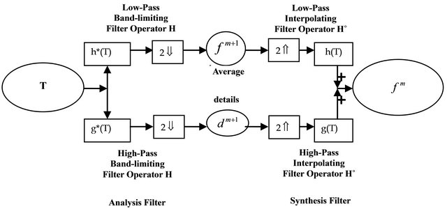
Figure 3. Sub-band coding scheme.
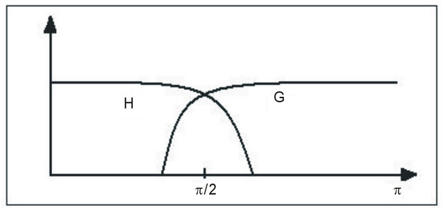
Figure 4. Magnitude responses of analysis filters.
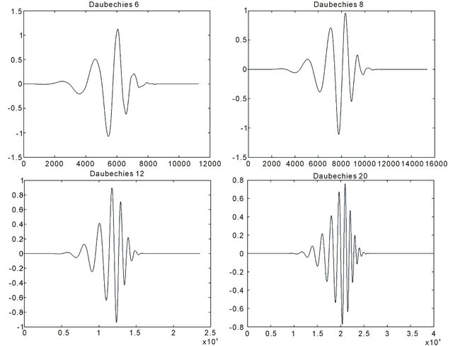
Figure 5. Some of the wavelets used in the research.
3) Backazimuth calculation The S-phase detection algorithm can also be categorized into three main modules:
1) Components Rotation 2) DTWT Processing that includes the following:
Ø Multiresolution Analysis
· Signal Decomposition (For radial and transverse components).
· Coefficients Reconstruction (For radial and transverse components).
3) Constructing the Composite Function of Transverse over Radial Amplitude Ratio.
3.2. P-Phase Detection Algorithm
It is known that the P-phase is linearly polarized with respect to the direction of propagation. Therefore, a metric that measures the degree of linear polarization is helpful to detect the P-phase arrival. Such a metric known as the rectilinearity function is defined by Kanasewich [22].
Its equation is:
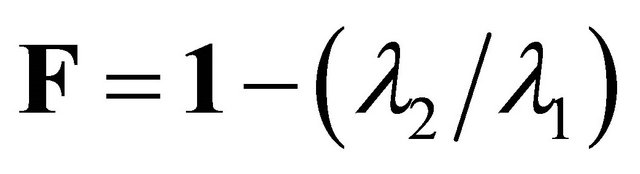 (3.1)
(3.1)
where  and
and  are the largest and the second largest eigenvalues of the covariance matrix respectively.
If the covariance matrix (Equation 3.2) is diagonalized, an estimate of the rectilinearity of particle motion trajectory over the specified time window can be obtained from the ratio of the principal axis of this matrix [22] i.e. the rectilinearity estimation can be obtained from the ratio of the largest and the second largest eigenvalues of the covariance matrix. The covariance matrix [23] is defined as:
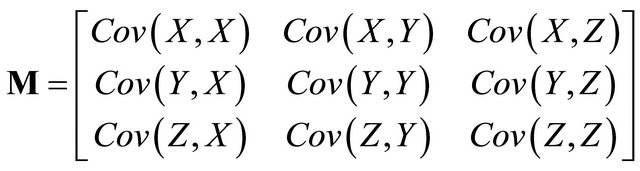 (3.2)
(3.2)
whereX: east component wavelet coefficients at scale j;
Y: north component wavelet coefficients at scale j;
Z: vertical component wavelet coefficients at scale j.
While the covariance of X and Y is defined as:
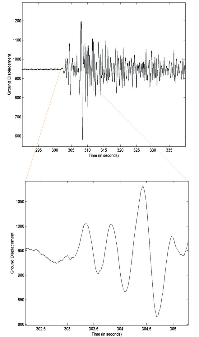
Figure 6. P-phase arrival of an earthquake record and the lower plot is a zoomed view of the arrival.
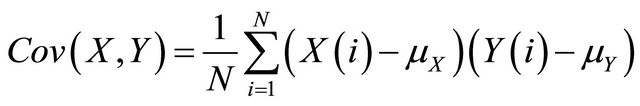 (3.3)
(3.3)
where  and
and  are the mean values of X and Y respectively.
The direction of polarization may be measured by considering the eigenvector of the largest principal axis [22]. If  is the largest eigenvalue and
  is the next largest eigenvalue of the covariance matrix, then a function of the form as in (Equation 3.1) would be close to

Figure 7. P-phase arrival of an earthquake record and a zoomed view of the arrival.
unity when rectilinearity is high ( ) and close to zero when two principal axes approach one another in magnitude (low rectilinearity).
The direction of polarization can be determined by considering the components of the eigenvector associated with the largest eigenvalue with respect to the coordinate directions X, Y and Z.
The P-phase algorithm is developed as can be described in the following steps:
1) Processing the three component seismic signals using Discrete Time Wavelet Transform (DTWT)
A three component seismic signals represented by east (X), north (Y) and vertical (Z) are processed by the discrete time wavelet transform (DTWT) to calculate the wavelet coefficients wc1, wc2 and wc3 respectively.
“Daubechies” wavelets are used in this process because of their compact support basis functions and their shape that coincide with seismic wave arrivals shapes.
Multiresolution Analysis
Each component is decomposed into several scales. So, the results are the wavelet coefficients x1j, x2j and x3j for east, north and vertical components respectively (j is the number of scales).
2) Constructing the rectilinearity function
At each scale, a pointwise moving window is constructed over the three components as shown in Figure 8.
The window length is determined using a measure called the varimax norm that is described in Appendix A. At each window, a 3-by-3 covariance matrix is constructed by using Equation (3.2) with x1j substituted for X, x2j substituted for Y and x3j substituted for Z. Then, eigenvalues and their corresponding eigenvectors are calculated.
At each window the rectilinearity function is constructed so that the result is a rectilinearity function (Fj) for each scale. Then, a composite rectilinearity function (Cf) is constructed so that the rectilinearity function of each scale contributes in this function. This composite function is constructed by (Equation 3.4).
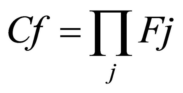 (3.4)
(3.4)
where j is the scale number.
The location where this function gets its maximum value is taken as the P-arrival time.
3) Calculating the back azimuth angle
Back-azimuth is the angle measured from north to the direction from which the energy arrives at a given station [24,25]. It is used to determine the longitudinal and transverse directions for an incoming ray at a prescribed station. For an incident P wave the backazimuth is calculated by constructing the rectilinearity function and finding the eigenvector associated with the maximum eigenvalue for the detected P-wave. This eigenvector repre-
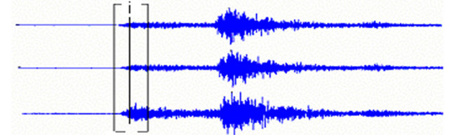
Nwin
Figure 8. Illustration of windowing used to calculate covariance matrices.
sents the direction of linear polarization that specifies the back azimuth angle. This calculation can be conducted at each wavelet scale as well as on the original signals. But, since the original three component signals generally contain noise, the calculation is carried out at the third and higher scales while the first two scales that contain high frequency noise are excluded. It is found that the polarization is conserved along different scales i.e. the same backazimuth angle is obtained in the different scales. So, one value is considered in the processing.
3.3. S-Phase Detection Algorithm
The S-phase is a shear wave with particle motion in the transverse direction [22]. Accordingly, it has higher amplitude in the transverse component relative to its amplitude in the radial or vertical component. So, in order to locate the S-phase arrival, the amplitude ratio of the transverse to radial components of the earthquake record is analyzed.
The S-phase algorithm is developed and can be described as follows:
1) Rotating the east and north components
The backazimuth angle  calculated in the previous part is used to rotate the east and north components to radial and transverse components respectively using the following equation:
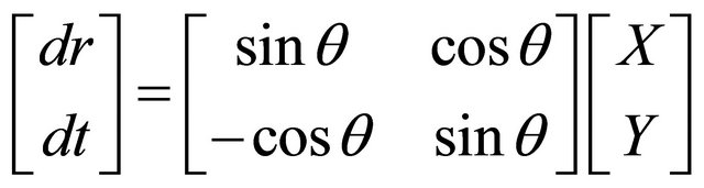 (3.5)
(3.5)
where dr and dt are the radial and transverse component respectively.
2) Processing the radial and transverse components by the discrete time wavelet transform (DTWT)
The radial and transverse components processed by the DTWT. So, the result is several scales for each component. Referring to the algorithm the result is xj and yj that represents the different scales for radial and transverse components respectively (j is the number of scales).
3) Constructing the amplitude ratio
At each scale, a transverse over radial amplitude ratio is calculated as follows:
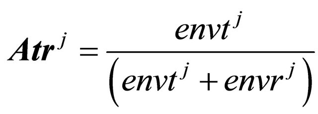 (3.6)
(3.6)
where envtj and envrj are the envelope functions of transverse and radial components respectively.
The envelope function is used to avoid divide-by-zero problems. It is defined as
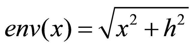 (3.7)
(3.7)
where h is the Hilbert transform of x.
All scales are combined to construct a second composite function (CT) to be used to locate the S-arrival.
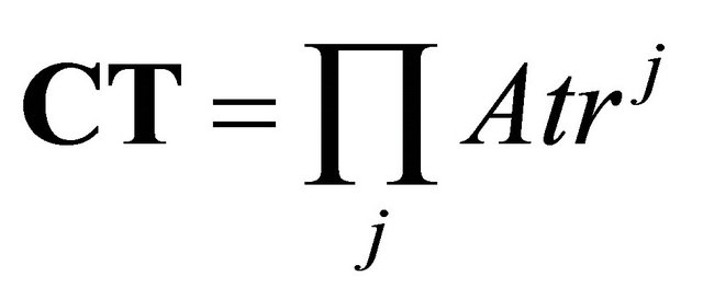 (3.8)
(3.8)
The point after the P arrival time that has a value that is at least one half the maximum of CT is chosen for the S arrival time. The peak of CT itself is not used because it represents the time when S-wave attains its highest amplitude which is few seconds after its arrival time [11].
Several wavelets are used in the wavelet transform decomposition because the choice of wavelet that used in the processing is very important in how well CT locates the S arrival time.
4. Results
4.1. Introduction
The algorithm has been tested by a real seismic data represented by several events recorded on various three components stations. The tested events apart from event 17 are distributed as shown in Figure 9. The Figure illustrates the tested events in orange circles as they located according to the stations in dark blue and black triangles for short period and broadband stations respectively. The purpose of this testing is to investigate if the project objectives listed in section 1 are achieved. To measure the performance of the algorithm, the algorithm results are compared with manual inspection results as well as with another automatic algorithm results (STA/ LTA method).
The performance of the system is measured by two ways: the first way is testing the ability of the software to detect P and S waves. However, the second way is comparing the results with another system results to see how accurate the system is.
4.2. P-Phase Detection Algorithm Results
The rectilinearity function proved to be an effective metric in locating the P-arrival time. Figure 10 shows the rectilinearity functions of six different scales obtained by testing the algorithm with event 21. It can be observed that the rectilinearity function is approximately equal to 1 when the waveform is linearly polarized and equal to zero when there is no linear polarization. This can be seen clearly in the first four scales.
Figure 11 shows the testing result of an earthquake (event 24). It illustrates the composite rectilinearity function Cf and how it is used to locate the P-arrival time.
Figure 12 shows the tested result of another earthquake (event 1) and the composite rectilinearity function Cf. It shows that the peak of this function is used to determine the P-arrival time. It can be observed from the figure that the position at this function is a maximum is where P-phase arrives.
Figure 13 illustrates the direction of Arabian Sea earthquake (event 4) as the result of testing the algorithm by three component data recorded by ABT station (one of the southern stations). Referring to Figure 9 it can be observed that ABT station is located in Southern Oman, which means that the algorithm indicates the event direction accurately as the event occurred in Arabian Sea.
In order to test the performance of the algorithm, it is
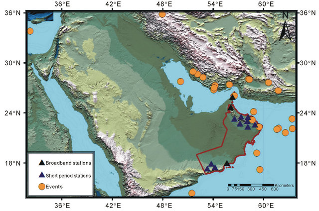
Figure 9. Distribution of tested events according to seismic stations.
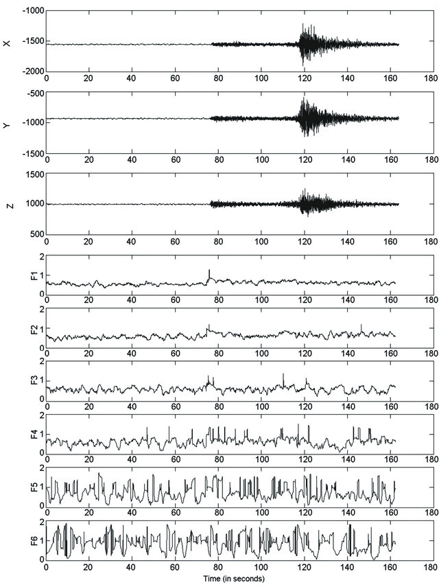
Figure 10. Three component waveforms of event 21 and its related rectilinearity functions of six different scales.

Figure 11. Three component data (east, north and vertical) of event 24 recorded by WBK station (one of the northern stations) with epicentral distance of 386.4 km and backazimuth of 106.9 degrees and the composite rectilinearity function Cf.
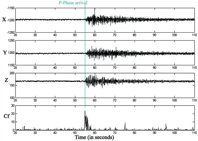
Figure 12. Three component data (east, north and vertical components) of event 1 recorded by JMD station with epicentral distance of 545.898 km and back azimuth of 96.03 degrees and the composite function Cf.

Figure 13. The direction of event 4 from ABT station.
tested by an event of magnitude 1.35 that occurs in California-Mexico border region (event 17). The purpose of this testing is to compare the algorithm results with the results obtained by another automatic detector and manual inspection that has been done by an analyst from the Broadband Array data collection center at the University of California, San Diego. The comparison between the analyst result and the algorithm result is illustrated in Figure 14. It can be noticed that the results are consistent with each other.
The three components signals illustrated in Figure 14 are recorded by a station with noisy local conditions (BVDA2 of ANZA network). That’s why; the STA/LTA (short term average/long term average) method couldn’t give a result for P-arrival time for the data recorded by this station. However, the P-phase detection algorithm gives a good result though of this noise condition.
The algorithm result is compared with the analyst result as well as with STA/LTA results. The comparison shows that the three results are consistent with each other as illustrated in Figure 15.
To enhance the algorithm results, they compared with the results of STA/LTA and analyst results of all the events listed in Table 1. The time difference in the arrival pick of the algorithm and that of the analyst is shown in Figure 16. It can be observed that the mean magnitude of algorithm error is low (0.1952 seconds) as compared with STA/LTA mean magnitude error (0.3982 seconds). This proves that the performance of the algorithm is efficient.
4.3. S-Phase Detection Algorithm Results
As stated earlier in Section 3, various wavelets are used in the wavelet transform decomposition. The wavelet is chosen to match the pattern of S-phase to provide the best match in the wavelet scales and thus give the composite function CT with the greatest dynamic range. Therefore, the composite function with the highest amplitude peak is used to locate the S-arrival.
The S-phase detection algorithm is tested by the same events used to test the P-phase detection algorithm. Its testing results of event 17 are compared with the analyst results as shown in Figure 17 while STA/LTA method failed to give any result for S-arrival.
Figures 18 and 19 show the results of testing the algorithm by two different events (event 4 and event 18 respectively). They illustrate the radial and transverse components and the composite function that constructed to be used to detect the S-arrival time. They show that the composite function of transverse to radial amplitude ratio accurately succeeded to determine the S-phase arrival as can be noticed from the figures that the peak of this function indicates the position where S-phase attains its highest magnitude while the onset time of S-phase is few seconds before this peak.
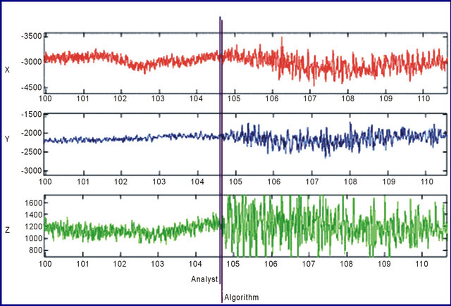
Figure 14. The three component signals of event 17 zoomed around P-arrival time to compare the analyst result with the algorithm result.
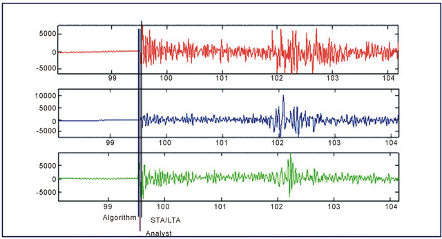
Figure 15. The result of comparing the algorithm with the analyst result and STA/LTA result when testing it by event 17 recorded by MONP station(Anza network) with epicentral distance of 10.656 km and backazimuth of 255.49 degrees.
Table 4. List of tested events.


Figure 16. Residual plot of P-Phase arrival.
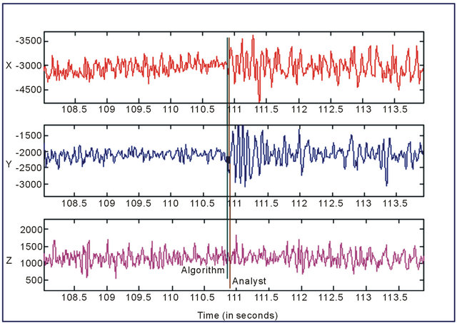
Figure 17. The three component signals of event 17 recorded by BVDA2 station with epicentral distance of 45.732 km and backazimuth of 353.73 degrees, zoomed around S-arrival time to compare the analyst result with the algorithm result.
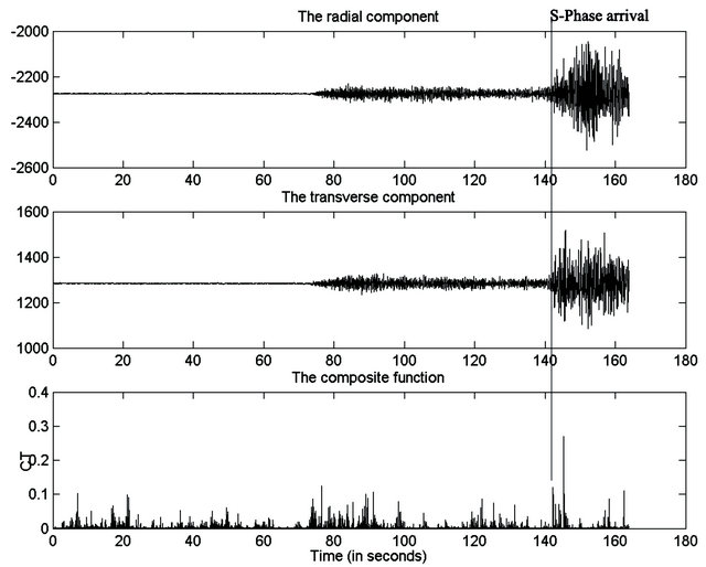
Figure 18. The radial and transverse components of event 4 recorded by ABT station with epicentral distance of 664.224 km and backazimuth of 43.9 degrees, and the composite function of the transverse to radial amplitude ratio.
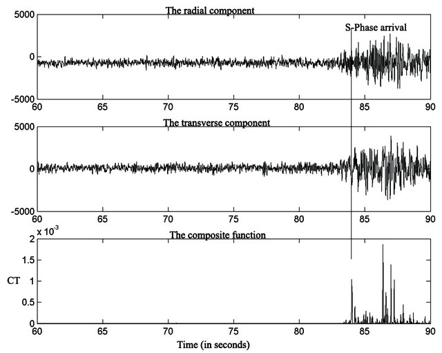
Figure 19. The radial and transverse components of event 18 recorded by BAN station (one of the broadband stations in northern Oman) with epicentral distance of 274.5 and backazimuth of 40.8 degrees and the composite function of transverse to radial amplitude ratio.
Figure 20 shows the residual plot of S-Phase arrival that illustrates the error between the algorithm and the analyst results (in circles) and the error between STA/ LTA results and the analyst results (in asterisks). It can be noticed that the mean magnitude error of the algorithm error is low (0.8197 seconds). In addition, it can be observed that there is no S-pick from STA/LTA for event 17 while the algorithm has good results and consistent with the analyst results.
As mentioned earlier in Section 4.3, several wavelets are independently used in the wavelet decomposition and the resulting CT of the highest dynamic range has been chosen to determine the S-arrival time. The results show that “Daubechies 8” wavelet is a good choice for most of the tested events. While the other wavelets such as “Daubechies 12” and “Daubechies 20” give good results for some events. This wavelet selection has been done according to the expected arrival shapes as described in details in Section 2.
5. Conclusions
Since the main objective of the project is to develop an algorithm that automatically detects particular classes of seismic wave, the software has been developed to detect P and S-phases in three component seismic data.
The algorithm has been tested by a real seismic data represented by multiple local and regional events recorded on various three components stations where it successfully detected P and S-phases.
Two important concepts have been presented in this research. The first concept is decomposing the signal into several resolutions or scales; important features in the seismic signals can be identified. Strong features in a signal can be maintained in several scales while weaker features will present in fewer scales or just one scale. The second concept is the wavelet type selection that depends on matching the wavelet to the arrival shapes.
The results of the software have been compared with a human analyst results as well as with the results obtained by software that uses STA/LTA (short term average/long term average) method. From the comparison results it can be concluded that the composite rectilinearity function and the composite function of transverse to radial amplitude ratio accurately determined P and S arrivals respectively. The results are consistent with the manual inspection results that done by an analyst as well as with other software based method in current professional use. The results showed that the STA/LTA failed to give any detection for S-phase of the tested events recorded by
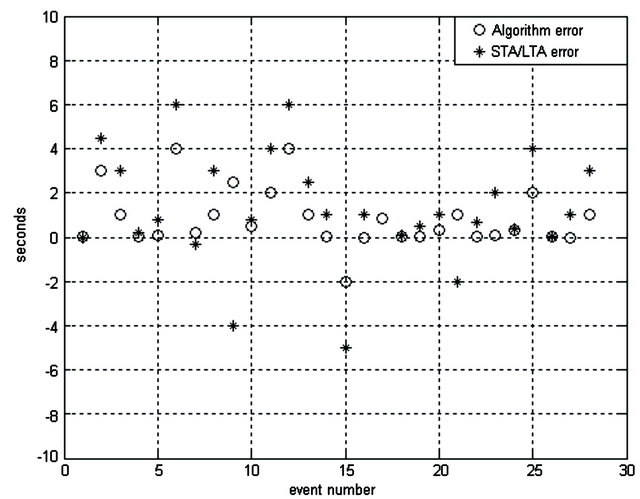
Figure 20. Residual plot of S-phase arrival.
stations with low signal to noise ratio conditions. In addition, the STA/LTA will fail to give a result for P-phase in low signal-to-noise conditions. However, the P and S-phase wavelet detection algorithms provided good results for P and S-arrivals and the results are consistent with the human analyst results.
To sum up, the developed wavelet algorithm can accurately determine the P and S arrivals in spite of the low signal-to-noise ratio. Furthermore, the software succeeded in determining back azimuths towards the earthquake sources.
The developed software can be used for a daily routine analysis in the seismological laboratories. In order to achieve this it should be tested by a huge amount of data set so that the parameters such as wavelet type that used in the DTWT analysis and the window size that used to construct the covariance matrices can be fixed.
6. Acknowledgements
Sincere thanks to Sultan Qaboos University for sponsoring this study. The first author would like to thank his colleagues at the earthquake monitoring center in Oman for sending the seismic data that are used in testing the software. In addition, many thanks to the staff at the Broadband Array data collection center, UCSD (http://eqinfo.ucsd.edu), for providing the seismic data that are used for results comparison. Partial support for this research was provided by NEHRP/USGS grants 03HQPA-0001 and 01HQAG0021. Furthermore, thanks to the University of Newcastle upon Tyne for providing computer facilities.
REFERENCES
- H. Dai and C. MacBeth, “Application of Back-Propagation Neural Networks to Identification of Seismic Arrival Types,” Physics of the Earth and Planetary Interiors, Vol. 101, No. 3-4, 1997, pp. 177-188. doi:10.1016/S0031-9201(97)00004-6
- H. Dai and C. MacBeth, “The Application of Back-Propagation Neural Network to Automatic Picking Seismic Arrivals from Single-Component Recordings,” Journal of Geophysical Research, Vol. 102, No. B7, 1997, pp. 15105- 15113. doi:10.1029/97JB00625
- R. Allen, “Automatic Phase Pickers: Their Present Use and Future Prospects,” Bulletin of the Seismological Society of America, Vol. 72, No. 68, 1982, pp. S225-S242.
- M. Baer and U. Kradolfer, “An Automatic Phase Picker for Local and Teleseismic Events,” Bulletin of the Seismological Society of America, Vol. 77, No. 4, 1987, pp. 1437-1445.
- A. Cichowicz, “An Automatic S-Phase Picker,” Bulletin of the Seismological Society of America, Vol. 83, No. 1, 1993, pp. 180-189.
- P. S. Earle and P. M. Shearer, “Characterization of Global Seismograms Using an Automatic-Picking Algorithm,” Bulletin of the Seismological Society of America, Vol. 84, No. 2, 1994, pp. 366-376.
- D. Patane and F. Ferrari, “ASDP: A PC-Based Program Using a Multi-Algorithm Approach for Automatic Detection and Location of Local Earthquakes,” Physics of the Earth and Planetary Interiors, Vol. 113, No. 1-4, 1999, pp. 57-74. doi:10.1016/S0031-9201(99)00030-8
- R. Sleeman and T. Van Eck, “Robust Automatic P-Phase Picking: An On-Line Implementation in the Analysis of Broadband Seismogram Recordings,” Physics of the Earth & Planetary Interiors, Vol. 113, No. 1-4, 1999, pp. 265-275.
- P.-J. Chung, M. L. Jost and J. F. Böhme, “Estimation of Seismic-Wave Parameters and Signal Detection Using Maximum Likelihood Methods,” Computers and Geosciences, Vol. 27, No. 2, 2001, pp. 147-156. doi:10.1016/S0098-3004(00)00088-1
- M. Tarvainen, “Automatic Seismogram Analysis: Statistical Phase Picking and Locating Methods Using OneStation Three-Component Data,” Bulletin of the Seismological Society of America, Vol. 82, No. 2, 1992, pp. 860- 869.
- K. S. Anant and F. U. Dowla, “Wavelet Transform Methods for Phase Identification in Three-Component Seismograms,” Bulletin of the Seismological Society of America, Vol. 87, No. 6, 1997, pp. 1598-1612.
- P. J. Oonincx, “A Wavelet Method for Detecting SWaves in Seismic Data,” Computational Geosciences, Vol. 3, No. 2, 1999, pp. 111-134. doi:10.1023/A:1011527009040
- H. Zhang, C. Thurber and C. Rowe, “Automatic P-Wave Arrival Detection and Picking with Multiscale Wavelet Analysis for Single-Component Recordings,” Bulletin of the Seismological Society of America, Vol. 93, No. 5, 2003, pp. 1904-1912. doi:10.1785/0120020241
- I. Daubechies, “Ten Lectures on Wavelets,” The Society of Industrial and Applied Mathematics, 1992.
- E. J. Stollnitz, T. D. DeRose and D. H. Salesin, “Wavelets for Computer Graphics, Theory and Applications,” Morgan Kaufmann, Burlington, 1996.
- G. Strang and T. Q. Nguyen, “Wavelets and Filter Banks,” Revised Edition, Wellesley-Cambridge Press, Wellesley, 1998.
- S. Mallat, “A Wavelet Tour of Signal Processing,” Academic Press, Waltham, 1999.
- S. Mallat, “A Theory for Multiresolution Signal Decomposition: The Wavelet Representation,” IEEE Transactions on Pattern Analysis and Machine Intelligence, Vol. 11, No. 7, 1989, pp. 674-493. doi:10.1109/34.192463
- B. Porat, “A Course in Digital Signal Processing,” John Wiley & Sons, Inc., Canada, 1997.
- M. Vetterli and C. Herley, “Wavelets and Filter Banks: Theory and Design,” IEEE Transactions on Signal Processing, Vol. 40, No. 9. 1992, pp. 2207-2232. doi:10.1109/78.157221
- M. Vetterli and D. Le Gall, “Perfect Reconstruction FIR Filter Banks: Some Properties and Factorizations,” IEEE Transactions on Acoustics, Speech and Signal Processing, Vol. 37, No. 7. 1989, pp. 1057-1071. doi:10.1109/29.32283
- E. R. Kanasewich, “Time Sequence Analysis in Geophysics,” University of Alberta Press, Edmonton, 1981.
- A. Jurkevics, “Polarization Analysis of Three-Component Array Data,” Bulletin of the Seismological Society of America, Vol. 78, No. 5, 1988, pp. 1725-1743.
- Stein, S. and M. Wysession, “An Introduction to Seismology, Earthquakes and Earth Structure,” Blackwell Publishing Ltd., Hoboken, 2003.
- K. Aki and P. G. Richards, “Quantitative Seismology,” University Science Books, Sausalito, 2002.
- R. Wiggins, “Minimum Entropy Deconvolution,” Geoexploration, Vol. 16, No. 1-2, 1978, pp. 21-35. doi:10.1016/0016-7142(78)90005-4
Appendix A
As mentioned in Section 3, a covariance matrix Mj[i] is calculated at each point I of x1j, x2j and x3j over a T point window. The size of window affects the eventual output, Cf. The aim is to obtain a function Cf that has a one main spike with a minimum of secondary spikes. There is a measure called the varimax norm [26] can be used for this purpose. The higher the varimax norm of a signal, the fewer spikes the signal has.
The varimax norm of the composite function Cf is calculated as:
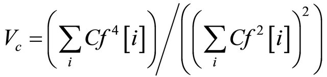
Thus, before selecting the size of the window (Nwin), several size windows are tested in order to maximize Vc. So, the window that gives a Cf with the highest varimax norm is selected as the window for a particular event.
Figure A1 and A2 show three component data of one of the tested events and a plot of the varimax norm versus the window size used to construct the covariance matrix. For this particular event, 6 seconds is chosen as the window length.

Figure A1. Three component data of an event.
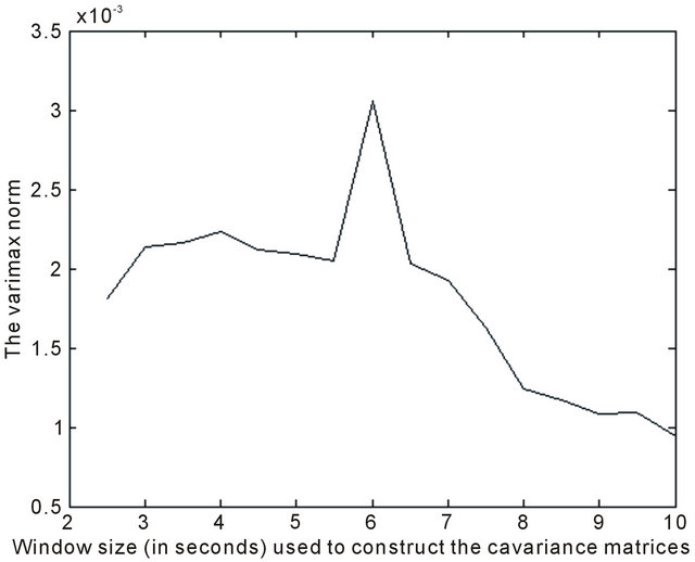
Figure A2. Demonstrating the effect of window size used to construct covariance matrices on the varimax norm of the composite rectilinearity function Cf.
Appendix B

Figure B1. Flow Chart of P-wave detection algorithm.
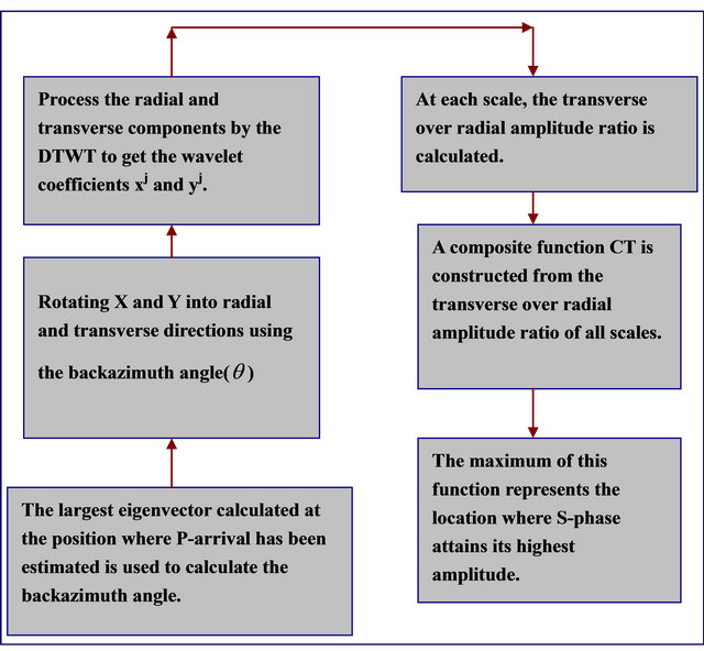
Figure B2. Flow Chart of S-wave detection algorithm.
NOTES
*Corresponding author.