Open Journal of Optimization
Vol.2 No.1(2013), Article ID:29423,8 pages DOI:10.4236/ojop.2013.21001
An Epsilon Half Normal Slash Distribution and Its Applications to Nonnegative Measurements
1Department of Mathematics and Statistics, University of Minnesota Duluth, Duluth, USA
2Department of Management Science, National Chiao Tung University, HsinChu, Chinese Taipei
3Department of EPLS, Florida State University, Tallahassee, USA
Email: *wgui@d.umn.edu, paulachen@g2.nctu.edu.tw, hw07d@fsu.edu
Received January 5, 2013; revised February 4, 2013; accepted February 28, 2013
Keywords: Epsilon Half Normal Distribution; Slash Distribution; Kurtosis; Skewness; Maximum Likelihood Estimation
ABSTRACT
We introduce a new class of the slash distribution using the epsilon half normal distribution. The newly defined model extends the slashed half normal distribution and has more kurtosis than the ordinary half normal distribution. We study the characterization and properties including moments and some measures based on moments of this distribution. A simulation is conducted to investigate asymptotically the bias properties of the estimators for the parameters. We illustrate its use on a real data set by using maximum likelihood estimation.
1. Introduction
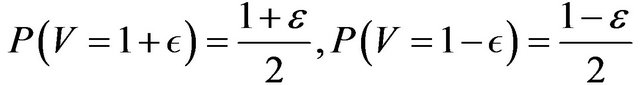
The epsilon half normal distribution, proposed by Castro et al. [1], is widely used for nonnegative data modeling, for instance, to consider the lifetime process under fatigue. We say that a random variable  has an epsilon half normal distribution with parameters
  and
and , denoted by
 , if its density function is given by, for
 ,
,
 (1)
(1)
where  denotes the standard normal density function. When
 , the epsilon half normal distribution reduces to the half normal distribution investigated in [2-4].
Castro et al. [1] provided mathematical properties of the epsilon half normal distribution and discussed some inferential aspects related to the maximum likelihood estimation.
On the other hand, a random variable  has a standard slash distribution
  with parameter
 , introduced in [5], if
  can be represented as
 (2)
(2)
where  and
and  are independent. It generalizes normality and has been much studied in the statistical literature.
For the limit case ,
,  yields the standard normal distribution
 . Let
. Let , the canonical slash distribution follows, see [6]. It is well known that the standard slash density has heavier tails than those of the normal distribution and has larger kurtosis. It has been very popular in robust statistical analysis and studied by some authors.
The general properties of this canonical slash distribution were studied in [5,7]. Kafadar [8] investigated the maximum likelihood estimates of the location and scale parameters.
Gómez et al. [9] replaced standard normal random variable  by an elliptical distribution and defined a new family of slash distributions. They studied its general properties of the resulting families, including their moments. Genc [10] proposed the univariate slash by a scale mixtured exponential power distribution and investigated asymptotically the bias properties of the estimators. Wang et al. [11] introduced the multivariate skew version of this distribution and examined its properties and inferences. They substituted the standard normal random variable
  by a skew normal distribution studied in [12] to define a skew extension of the slash distribution.
Olmos et al. [3] introduced the slashed half normal distribution by a scale mixtured half normal distribution and showed that the resulting distribution has more kurtosis than the ordinary half normal distribution. Since the epsilon half normal distribution  is an extension of the half normal distribution, it is naturally to define a slash distribution based on it in which skewness and thick tailed situations may exist. It leads to a new model on nonnegative measurements with more flexible asymmetry and kurtosis parameters.
The paper is organized as follows: in Section 2, we introduce the new slash distribution and study its relevant properties, including the stochastic representation etc. In Section 3 we discuss the inference, moments and maximum likelihood estimation for the parameters. Simulation studies are performed to investigate the behaviors of estimators in Section 4. In Section 5, we give a real illustrative application and report the results. Section 6 concludes our work.
2. Epsilon Half Normal Slash Distribution
2.1. Stochastic Representation
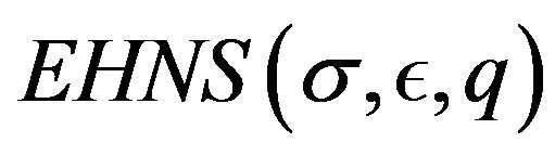
Definition 2.1 A random variable  has an epsilon half normal slash distribution if it can be represented as the ratio
 (3)
(3)
where  defined in (1) and
 are independent,
  ,
,  ,
, . We denote it as
 .
.
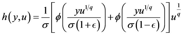
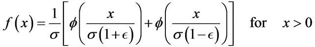
Proposition 2.2 Let . Then, the density function of
  is given by, for
 ,
,
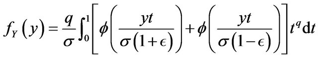 (4)
(4)
where ,
,  ,
, .
.
Proof. From (1), the joint probability density function of  and
and  is given by, for
 ,
,

Using the transformation:
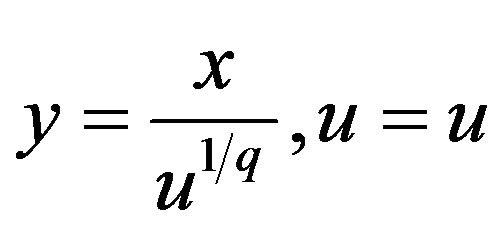 the joint probability density function of
  and
and  is given by, for
 ,
,
The marginal density function of  is given by

After changing the variable into , the dendity function will be obtained as stated.
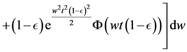
Remark 2.3 If , the density function (4) reduces to
which is the density function for the slashed half normal distribution studied by [3]. As ,
,

The limit case of the epsilon half normal slash distribution is the epsilon half normal distribution. For , the canonical case follows.
Figure 1 shows some plots of the density function of the epsilon half normal slash distribution with various parameters.
The cumulative distribution function of the epsilon half normal slash distribution  is given as follows. For
 ,
,
 (5)
(5)
where  is the cumulative distribution function for the standard normal random variable.
Proposition 2.4 Let 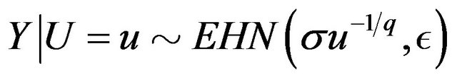 and
and , then
 .
.

Figure 1. The density function of  with various parameters.
Proof.

Remark 2.5 Proposition 2.4 shows that the epsilon half normal slash distribution can be represented as a scale mixture of an epsilon half normal distribution and uniform distribution. The result provides another way besides the definition (3) to generate random numbers from the epsilon half normal slash distribution
 .
.
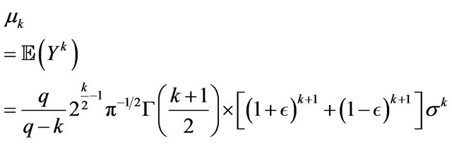
2.2. Moments and Measures Based on Moments
In this section, we derive the moment generating function,the k-th moment and some measures based on the moments.
Proposition 2.6 Let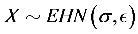 , then the moment generating function of
  is given by for
 ,
,
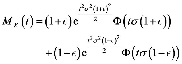 (6)
(6)
where  and
and . Proof. See [1].
Proposition 2.7 Let , then the moment generating function of
  is given by, for
 ,
,
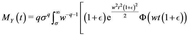 (7)
(7)
 (8)
(8)
where ,
,  and
and .
.
Proof. From Proposition 2.4 and using properties of the conditional expectation, we have
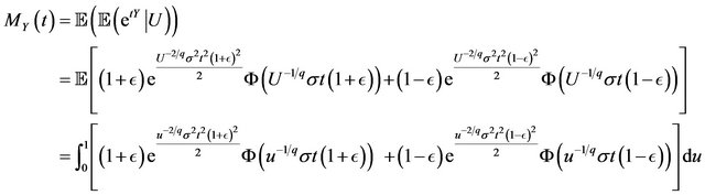
Making the transformation  and the result follows.
Proposition 2.8 Let , then the
  non-central moments are given by
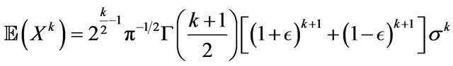 (9)
(9)
for . where
  and
and .
.
Proof. See [1].
Proposition 2.9 Let , where
 ,
,  and
and . For
. For  and
and , the
, the  non-central moment of
  is given by
 (10)
(10)
Proof. From the stochastic representation defined in (3) and the results in (9), the claim follows in a straightforward manner.

The following results are immediate consequences of (10).
Corollary 2.10 Let , where
 ,
,  and
and . The mean and variance of
  are given by
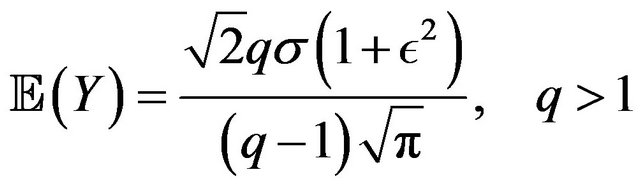 (11)
(11)
and for ,
,

For the standardized skewness
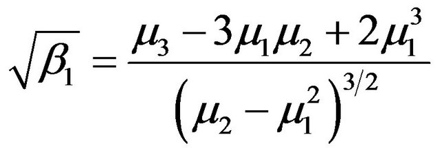
and kurtosis coefficients
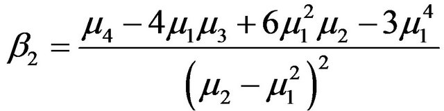 we have the following results.
Corollary 2.11 Let , where
 ,
,  and
and . The skewness and kurtosis coefficients of
  are given by
 (12)
(12)
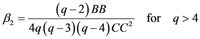 (13)
(13)
where


Remark 2.12 As , the skewness coefficient converges.
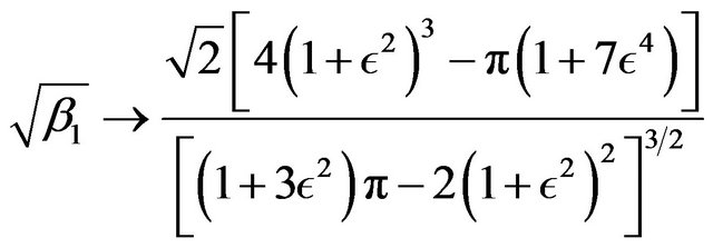
and the kurtosis coefficient converges as well
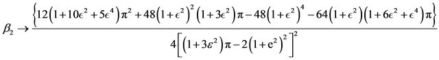
which are the corresponding skewness and kurtosis coefficients for the epsilon half normal distribution .
.
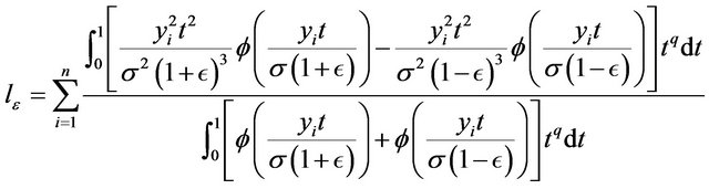
Figure 2 shows the skewness and kurtosis coefficients with various parameters for the  model. The skewness and kurtosis coefficients decrease as
  increases. The parameter
  does not affect the two coefficents.
3. Maximum Likelihood Inference
In this section, we consider the maximum likelihood estimation about the parameters of the  model defined in (4). For
 ,
,

where .
.
Suppose  is a random sample of size
  from the epsilon half normal slash distribution
 . Then the log-likelihood function can be written as
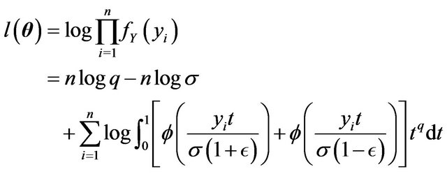 (14)
(14)
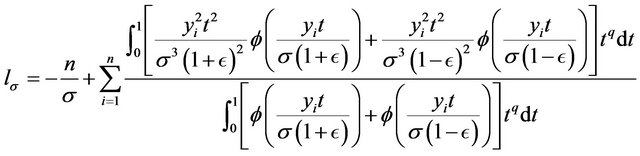
The estimates of the parameters maximize the likelihood function. By taking the partial derivatives of the log-likelihood function with respect to  respectively and equalizing the obtained expressions to zero, we obtain the following maximum likelihood estimating equations.
 (a)
(a) (b)
(b)
Figure 2. The plot for the skewness 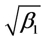 and kurtosis coefficient
  with various parameters. a) Skewness coefficient; b) Kurtosis coefficient.

The maximum likelihood estimating equations above are not in a simple form. In general, there are no implicit expression for the estimates. The estimates can be obtained through some numerical procedures such as Newton-Raphson method. Many programs provide routines to solve such maximum likelihood estimating equations.
In this paper, all the computations are performed using software R. The MLE estimators are computed by the optim function which uses L-BFGS-B method. In the following section, a simulation is conducted to illustrate the behavior of the MLE.
For asymptotic inference of , the Fisher information matrix
  plays a key role. It is well known that its inverse is the asymptotic variance matrix of the maximum likelihood estimators. For the case of a single observation
 , we take the second order derivatives of the log-likelihood function in (14) and the Fisher information matrix is defined as
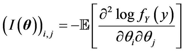 (15)
(15)
for  and
and .
.
Proposition 3.1 Let  is a random sample of size
  from the distribution
 , where
  and
and  is the maximum likelihood estimator of
 , we have
 (16)
(16)
Proof. It follows directly by the large sample theory for maximum likelihood estimators and the Fisher information matrix given above.
4. Simulation Study
4.1. Data Generation
In this section, we present how to generate the random numbers from the epsilon half normal slash distribution .
.
Proposition 4.1 Let  be two independent random variables, where
  and
and  is such that
then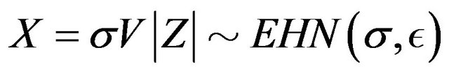 , where
  and
and  .
.
Proof. For ,
,

The density function of  is
is
which proves the result.
Using the definition in (3) and the results in Proposition 4.1, we can generate variates from the epsilon half normal slash distribution  with the following algorithm.
Algorithm 4.2 Using the definition in (3) to generate data
• Generate ,
,  and
and
• 
• Let  if
if . Otherwise
• Set 
• Set 
4.2. Behavior of MLE
In this section, we perform a simulation study to illus trate the behavior of the MLE estimators for parameters ,
,  and
and .
.
It is known that as the sample size increases, the distribution of the MLE tends to the normal distribution with mean  and covariance matrix equal to the inverse of the Fisher information matrix. However, the log-likelihood function given in (14) is a complex expression. It is not generally possible to derive the Fisher information matrix. Thus, the theoretical properties (asymptotically normal, unbiased etc) of the MLE estimators are not easily derived. We study the properties of the estimators numerically.
We first generate 500 samples of size  and
and  from the
  distribution for fixed parameters. The estimators are computed by the optim function which uses L-BFGS-B method in software R. The empirical means and standard deviations(SD) of the estimators are presented in Table 1.
It can be seen from Table 1 that the parameters are well estimated and the estimates are asymptotically un-
Table 1. Empirical means and SD for the MLE estimators of ,
,  and
and .
.
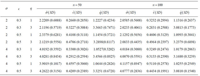
Table 2. Summary for the life of fatigue fracture.
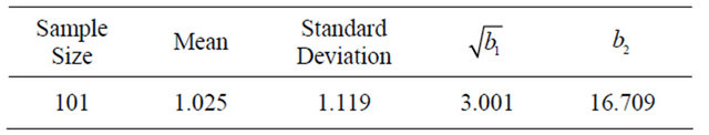
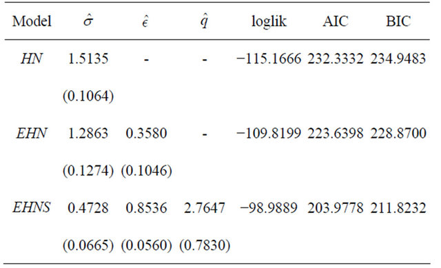
Table 3. Maximum likelihood parameter estimates(with (SD)) of the HN, EHN and EHNS models for the stressrupture data.
biased. The empirical mean square errors decrease as sample size increases as expected.
5. Real Data Illustration
In this section, we consider the stress-rupture data set, the life of fatigue fracture of Kevlar 49/epoxy that are subject to the pressure at the 90% level. The data set has been previously studied in [1,3,13,14].
Table 2 summarizes descriptive statistics of the data set where  and
and  are sample asymmetry and kurtosis coefficients, respectively. This data set indicates non negative asymmetry.
We fit the data set with the half normal, the epsilon half normal and the epsilon half normal slash distributions using maximum likelihood method. The results are reported in Table 3. The usual Akaike information criterion (AIC) and Bayesian information criterion (BIC) to measure of the goodness of fit are also computed.  and
and . where
  is the number of parameters in the distribution and
  is the maximized value of the likelihood function. The results indicate that
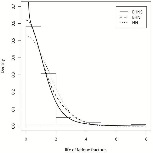
  model fits best. Figures 3(a) and (b) display the fitted models using the MLE estimates.
6. Concluding Remarks
In this article, we have studied the epsilon half normal slash distribution . It is defined to be the quotient of two independent random variables, an epsilon half normal random variable and a power of the uniform distribution. This nonnegative distribution extends the
 (a)
(a)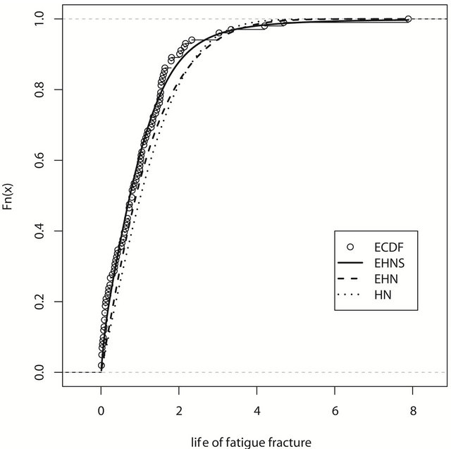 (b)
(b)
Figure 3. Models fitted for the life of fatigue fracture data set. a) Histogram and fitted curves; b) Empirical and fitted CDF.
epsilon half normal, the half normal distribution etc. Probabilistic and inferential properties are derived. A simulation is conducted and demonstrates the good performance of the maximum likelihood estimators. We apply the model to a real dataset and the results demonstrate that the proposed model is very useful and flexible for non negative data.
7. Acknowledgements
The authors would like to thank the anonymous reviewers and the editor for their valuable comments and suggestions to improve the quality of the paper.
REFERENCES
- L. Castro, H. Gómez and M. Valenzuela, “Epsilon Half-Normal Model: Properties and Inference,” Computational Statistics & Data Analysis, Vol. 56, No. 12, 2012, pp. 4338-4347. Hdoi:10.1016/j.csda.2012.03.020
- A. Pewsey, “Improved Likelihood Based Inference for the General Half-Normal Distribution,” Communications in Statistics—Theory and Methods, Vol. 33, No. 2, 2004, pp. 197-204. Hdoi:10.1081/STA-120028370
- N. Olmos, H. Varela, H. Gómez and H. Bolfarine, “An Extension of the Half-Normal Distribution,” Statistical Papers, Vol. 53, No. 4, 2011, pp. 1-12.
- M. Wiper, F. Girón and A. Pewsey, “Objective Bayesian Inference for the Half-Normal and Half-t Distributions,” Communications in Statistics—Theory and Methods, Vol. 37, No. 20, 2008, pp. 3165-3185. Hdoi:10.1080/03610920802105184
- W. Rogers and J. Tukey, “Understanding Some LongTailed Symmetrical Distributions,” Statistica Neerlandica, Vol. 26, No. 3, 1972, pp. 211-226. Hdoi:10.1111/j.1467-9574.1972.tb00191.x
- N. Johnson, S. Kotz and N. Balakrishnan, “Continuous Univariate Distributions,” Wiely, Hoboken, 1995.
- F. Mosteller and J. Tukey, “Data Analysis and Regression: A Second Course in Statistics,” Addison-Wesley Pub. Co., Boston, 1977.
- K. Kafadar, “A Biweight Approach to the One-Sample Problem,” Journal of the American Statistical Association, Vol. 77, No. 378, 1982, pp. 416-424. Hdoi:10.1080/01621459.1982.10477827
- H. Gómez, F. Quintana and F. Torres, “A New Family of Slash-Distributions with Elliptical Contours,” Statistics & Probability Letters, Vol. 77, No. 7, 2007, pp. 717-725. Hdoi:10.1016/j.spl.2006.11.006
- A. Genc, “A Generalization of the Univariate Slash by a Scale-Mixtured Exponential Power Distribution,” Communications in Statistics—Simulation and Computation, Vol. 36, No. 5, 2007, pp. 937-947. Hdoi:10.1080/03610910701539161
- J. Wang and M. Genton, “The Multivariate Skew-Slash Distribution,” Journal of Statistical Planning and Inference, Vol. 136, No. 1, 2006, pp. 209-220. Hdoi:10.1016/j.jspi.2004.06.023
- A. Azzalini, “A Class of Distributions Which Includes the Normal Ones,” Scandinavian Journal of Statistics, Vol. 12, No. 2, 1985, pp. 171-178.
- D. Andrews and A. Herzberg, “Data: A Collection of Problems from Many Fields for the Student and Research Worker,” Vol. 18, Springer-Verlag, New York, 1985.
- R. Barlow, R. Toland and T. Freeman, “A Bayesian Analysis of the Stress-Rupture Life of Kevlar/Epoxy Spherical Pressure Vessels,” In: C. Clarotti and D. Lindley, Eds., Accelerated Life Testing and Experts Opinions in Reliability, Elsevier Science Ltd., Amsterdam, 1988, pp. 203-236.
NOTES
*Corresponding author.