ABSTRACT

In this paper, we shall be interested in characterization of efficient solutions for special classes of problems. These classes consider roughly B-invexity of involved functions. Sufficient and necessary conditions for a feasible solution to be an efficient or properly efficient solution are obtained.

1. Introduction

The study of multi-objective programming problems was very active in recent years. The minimum (efficient, Pareto) solution is an important concept in mathematical models, economics, decision theory, optimal control and game theory (see, for example, [1]). In most works, an assumption of convexity was made for the objective functions. Very recently, some generalized convexity has received more attention (see, for example, [2-6]). A significant generalization of convex functions is invex function introduced first by Hanson [7], which has greatly been applied in nonlinear optimization and other branches of pure and applied sciences.

The concept of B-invex functions was proposed by [8] as generalization of convex functions; these functions were extended to quasi B-invex, and pseudo B-invex functions. Many functions seem to be B-invex, but they are not, and many non B-invex functions are able to get B-invex by choosing a suitable condition. Based on the previous discussion, Tarek [9] introduced a new class of B-invex functions, this class called roughly B-invex functions.

Inspired and motivated by above works, the purpose of this paper is to formulate a multi-objective programming problem which it involves roughly B-invex functions. An efficient solution for considered problem is characterized by weighting and ε-constraint approaches. In the end of the paper, we obtain sufficient and necessary conditions for a feasible solution to be an efficient or properly efficient solution for this kind of problems. Let us survey, briefly, the definitions and some results of roughly B-invexity.

Definition 1 [10]

Let. The set M is said to be B-invex with respect to at if there exists

such that, for each, and.

M is said to be B-invex set with respect to η if M is B-invex at each with respect to the same η.

Note that, as in convex set, the intersection of finite (or infinite) family of B-invex sets is B-invex but the union is not necessarily B-invex set. Also, the sum of B-invex sets and the multiplying a B-invex set by a real number are again B-invex sets. Every B-invex set with respect to is an invex set when b = 1; but the converse is not necessarily true.

Definition 2 [9]

A numerical function f , defined on a B-invex subset M of Rⁿ, is said to be roughly B-invex with respect to with roughness degree r at if there exists, such that

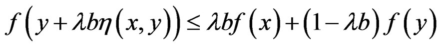for each, and such that.

f is said to be roughly B-invex on M with respect to if it is roughly B-invex at each with respect to the same.

Every invex function, with respect to η is roughly B-invex function with respect to same η, where b (x, y) = 1; but the converse is not necessarily true. If the functions are all roughly B-invex with respect to with roughness degree on a B-invex set, then the function

is roughly B-invex with respect to same η with roughness degree

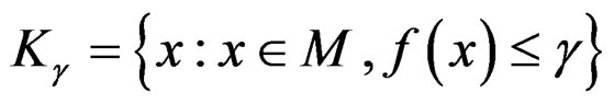
on M for a_i ≥ 0. If is roughly B-invex with respect to with roughness degree r, on B-invex set, then for any real number the level set is B-invex set. A numerical function f defined on a B-invex set is roughly B-invex function with respect to with roughness degree r if and only if epi(f) is a B-invex set. If is a family of numerical functions, which are roughly B-invex with respect to with roughness degree r and bounded from above on a B-invex set, then the numerical function

is a roughly B-invex with respect to same η with roughness degree r on M. If is a differentiable roughly B-invex function with respect to with roughness degree r, at, then there exists a function, such that

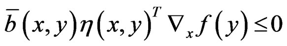
for each such that.

Definition 3 [9]

A numerical function f, defined on a B-invex subset M of Rⁿ, is said to be quasi roughly B-invex with respect to with roughness degree r at, if there exists, such that

for each, and such that.

f is said to be quasi roughly B-invex on M with respect to if it is roughly B-invex at each with respect to the same.

A is quasi roughly B-invex with respect to η: M × M → Rⁿ with roughness degree r, on, if and only if the level set

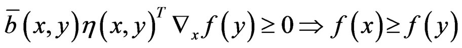
is B-invex set. A roughly B-invex function, with respect to with roughness degree r is quasi roughly B-invex function with respect to same η with roughness degree r. Let be B-invex set, if is differentiable quasi roughly B-invex with respect to with roughness degree r, at, then there exists a function, such that

for each such that.

Definition 4 [9]

A numerical function f, defined on a B-invex subset M of Rⁿ, is said to be pseudo roughly B-invex with respect to with roughness degree r at, if there exists, and, there exists a strictly positive function a: Rⁿ × Rⁿ → R such that

for each such that.

If is roughly B-invex function with respect to with roughness degree r on B-invex set, then f is pseudo roughly B-invex function with respect to same η with roughness degree r on M. Let be B-invex set and be a differentiable pseudo roughly B-invex with respect towith roughness degree r, at, then there exists a function, such that

for each such that.

2. Problem Formulation

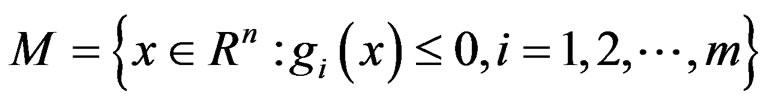
Let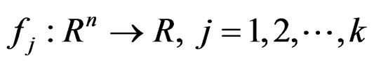, and 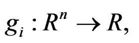i = 1, 2, ···, m are real valued roughly B-invex functions on Rⁿ. A roughly B-invex multi-objective programming problem is formulated as follows:

(P)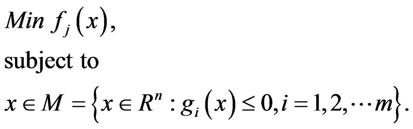

Definition 5 [11]

A feasible solution x for (P) is said to be an efficient solution for (P) if and only if there is no other feasible x for (P) such that, for some,

.

Definition 6 [11]

An efficient solution for (P) is a properly efficient solution for (P) if there exists a scalar such that for each, and each satisfying, there exists at least one with and

.

Lemma 1 [9]

If is roughly B-invex with respect to with roughness degree r, on Rⁿ, i = 1, 2, ···, m, then the set

is B-invex set.

Lemma 2 [9]

If is quasi roughly B-invex with respect to with roughness degree r, on Rⁿ, i = 1, 2, ···, m, then the set

is B-invex set.

Lemma 3

Let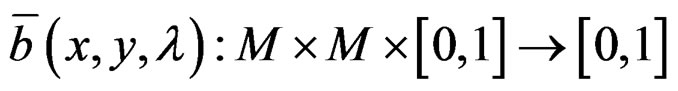. If is a roughly B-invex function with respect to with roughness degree r on a B-invex set, then the set

is convexwhere.

Proof. Let then for and we have

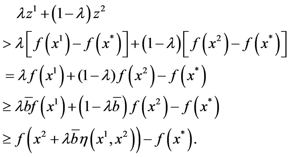
Since f is a roughly B-invex function on a B-invex set M. Then, and hence A is convex set.

For a feasible point, we denote as the index set for binding constraints at x^*, i.e.,.

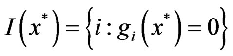3. Characterizing Efficient Solutions by Weighting Approach

To characterizing an efficient solution for problem (P) by weighting approach [11] let us scalarize problem (P) to become in the form.

(P_w)    , s.t.where     

and, j = 1, 2, ···, k are roughly B-invex with respect to with roughness degree r_j on B-invex set M.

Theorem 1

If is an efficient solution for problem (P), then there exist

such that is an optimal solution for problem (P_w).

Proof. Let be an efficient solution for problem (P), then the system j = 1, 2, ···, k has no solution. Upon Lemma 3 and by applying the generalized Gordan theorem [12], there exist such that

and       .

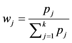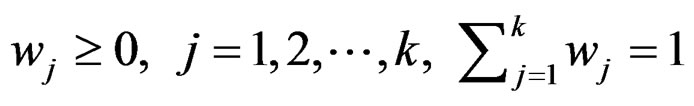Denote           then       and          .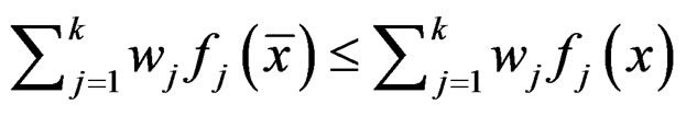

Hence is an optimal solution for problem (P_w).

Theorem 2

If is an optimal solution for corresponding to, then is an efficient solution for problem (P) if either one of the following two conditions holds:

(i) for all; or (ii) is the unique solution of.

Proof. To proof see V. Chankong, Y. Y. Haimes [11].

4. Characterizing Efficient Solutions by ε-Constraint Approach

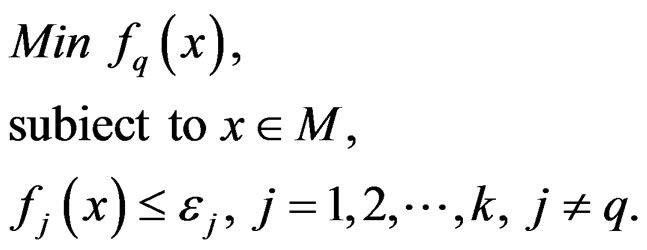
An ε-constraint approach is one of the common approaches for characterizing efficient solutions of multiobjective programming problems [11]. In the following we shall characterizing an efficient solution for multiobjective roughly B-invex programming problem (P) in term of an optimal solution of the following scalar problem.

where are roughly B-invex with respect to with roughness degree r_j on B-invex set M.

Theorem 3

If is an efficient solution for problem (P), then is an optimal solution for problem corresponding to.

wang#title3_4:spProof.

Let be not optimal solution for where So there exists

such that        ,

.

Thus, is inefficient solution for problem (P) which is a contradiction. Hence is an optimal solution for problem.

Theorem 4

Let is an optimal solution of for all  q = 1, 2, ···, k, where, j = 1, 2, ···, k . Then is an efficient solution for problem (P).

wang#title3_4:spProof.

Since is an optimal solution for, for all q = 1, 2, ···, k. So, for each, we get q = 1, 2, ···, k.

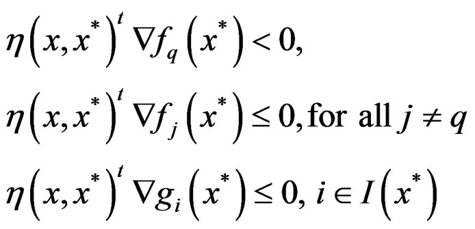
This implies that the system j = 1, 2, ···, k has no solution, i.e. is an efficient solution for problem (P).

5. Sufficient and Necessary Conditions for Efficiency

In this section, we discuss the sufficient and necessary conditions for a feasible solution x^* to be efficient or properly efficient for problem (P) in the form of the following theorems.

Theorem 5

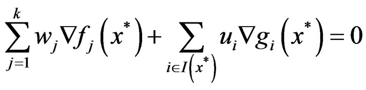
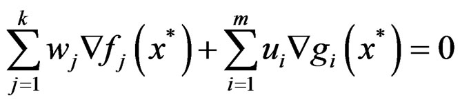
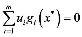
Suppose there exists a feasible solution x^* for (P), and scalars, such that

. (1)

If, j = 1, 2, ···, k are roughly B-invex with respect to with roughness degree r at x^* and g_i, is roughly B-invex with respect to same η with roughness degree r_i at x^*. Then x^* is a properly efficient solution for problem (P).

Proof.

Since, j = 1, 2, ···, k and are roughly B-invex with respect to same η, then there exists a function such that

by (1) for each such that

.

Thus, for all, which implies that x^* is the minimizer of

such that        

under the constraint where. Hence, from Theorem (4.11) of [11], x^* is a properly efficient solution for problem (P).

Theorem 6 Let x^* be a feasible solution for (P). If there exist scalars,

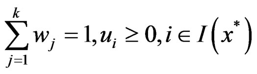such that the triplet (x^*, w_i, u_i) satisfies (1) of Theorem (5),

is strictly roughly B-invex with respect to η: M × M → Rⁿ with roughness degree r at x^* and g_i, is roughly B-invex with respect to same η with roughness degree r_i at x^*. Then x^* is an efficient solution for problem (P).

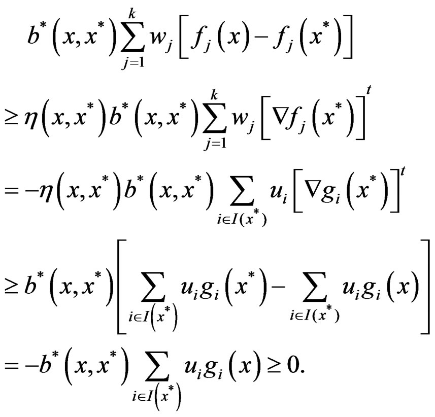
Proof.

Suppose that x^* is not an efficient solution for (P). Then, there exists a feasible, and index v such that

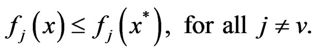
Since             

is strictly roughly B-invex with respect to η with roughness degree r at x^*, then there exists a function such that

. (2)

Also, roughly B-invexity of g_i, with respect to same η at x^* with roughness degree r_i implies

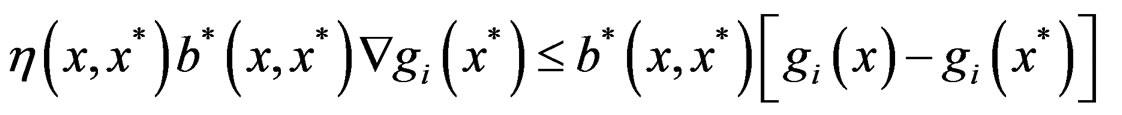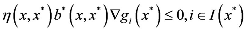i.e.    ,     (3)

such that. Adding (2) and (3), contradicts (1). Hence, x^* is an efficient solution for problem (P).

Remark 1

Similarly as in Theorem (5), it can be easily seen that x^* becomes properly efficient solution for (P), in the above theorem, if w_j > 0, for all j = 1, 2, ···, k.

Theorem 7

Suppose there exists a feasible solution x^* for (P), and scalars w_i > 0, j = 1, 2, ···, k, such that (1) of Theorem (5) holds. If

is pseudo roughly B-invex with respect to with roughness degree r at x^* and g_I is quasi roughly B-invex with respect to same η with roughness degree r_I at x^*. Then x^* is a properly efficient solution for problem (P).

Proof.

Since, and g_I are quasi roughly B-invex with respect to η with roughness degree r_I at, then there exists a function such that

for all such that. By using (1)we have  

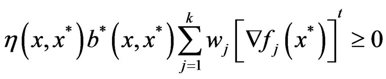
which implies

since                

is pseudo roughly B-invex with respect to same η with roughness degree r at x^* which implies that x^* is the minimizer of

such that       

under the constraint where ≥ max(r, r_i). Therefore, x^* is a properly efficient solution for problem (P).

Theorem 8

Suppose that there exist a feasible solution x^* for (P) and scalars,

, such that (1) of Theorem (5) holds. Let

be strictly pseudo roughly B-invex with respect to with roughness degree r at and g_I be quasi  roughly B-invex with respect to same η with roughness degree r_I at x^*. Then x^* is an efficient solution for problem (P).

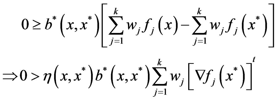
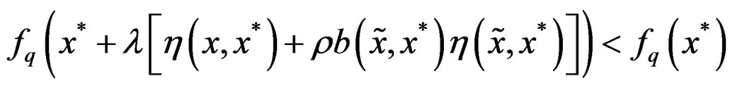
Proof. Suppose that x^* is not an efficient solution for (P).Then, there exists a feasible x for (P), and index v such that then there exists a function such that,

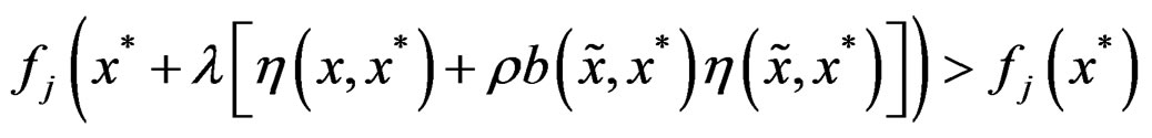
Strictly pseudo roughly B-invexity of

implies that

for all such that. Since g_I is quasi roughly B-invex with respect to same η with roughness degree r_I at andthen         for all such that

.

The proof now similar to the proof of Theorem (6).

Remark 2

Similarly as in Theorem (7), it can be easily seen that x^* becomes properly efficient solution for (P), in the above theorem, if.

Theorem 9

Suppose there exists a feasible solution x^* for (P), and scalars such that (1) of Theorem (5) holds. Let

be pseudo roughly B-invex with respect to with roughness degree at x^* and be quasi roughly B-invex with respect to same η with roughness degree at x^*. Then x^* is a properly efficient solution for problem (P).

Proof. The proof is similar to the proof of Theorem (7).

Theorem 10

Suppose that there exist a feasible solution x^* for (P) and scalars,

such that (1) of Theorem (5) holds. If,

is quasi roughly B-invex with respect to with roughness degree r at x^* and is strictly pseudo roughly B-invex with respect to same η with roughness degree r_I at x^*. Then x^* is an efficient solution for problem (P).

Proof. The proof is similar to the proof of Theorem (8).

Remark 3

Similarly as in Theorem (7), it can be easily seen that x^* becomes properly efficient solution for (P), in the above theorem, if.

Theorem 11 (Necessary Optimality Criteria)

Assume that x^* is a properly efficient solution for problem (P). Assume also that there exist a feasible point for (P) such that, and each is roughly B-invex with respect to η: M × M → Rⁿ with roughness degree r_i at x^*. Then, there exists scalars and, such that the triplet satisfies

. (4)

Proof. Let the following system

. (5)

has a solution for every. Since by the assumed Slater-type condition,

and then from roughly B_i-invexity of g_i at with respect to η, there exists a function such that

. (6)

Therefore from (5) and (6)

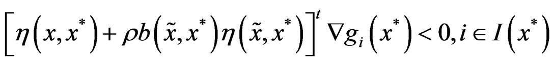for all. Hence for some positive λ small enough

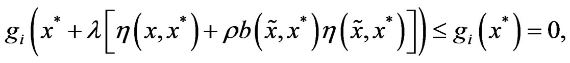
Similarly, for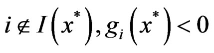, and for small enough

.

Thus, for λ sufficiently small and all

is feasible for problem (P). For sufficiently small, (5) gives

. (7)

Now, for all such that

(8)

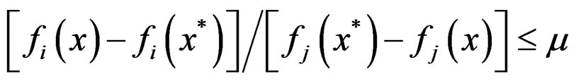
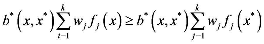
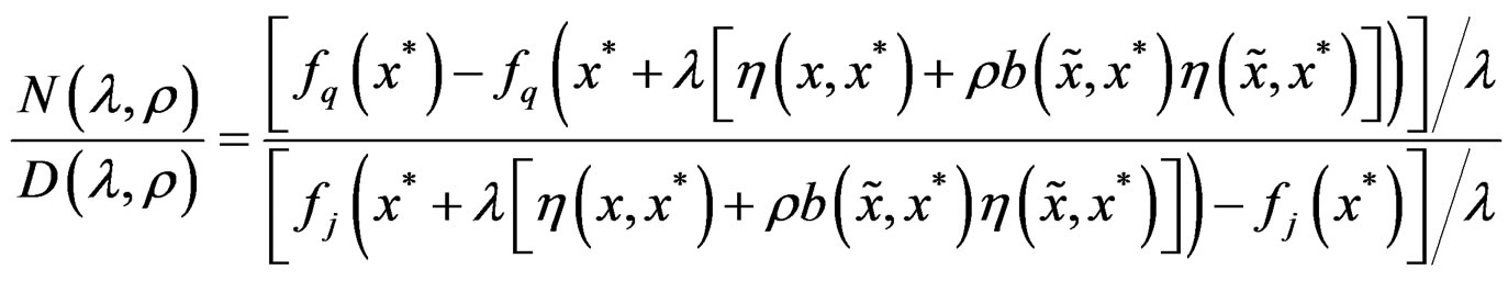
Consider the ratio (see Equation (9))

From (5),. Similarly,; but, by (8).

Thus, the ratio in (9) becomes unbounded, contradicting the proper efficiency of x^* for (P). Hence, for each q = 1, 2, ···, k, the system (5) has no solution. The result then follows from an application of the Farkas Lemma as in [12], namely

.

Theorem 12

Assume that x^* is an efficient solution for problem (P) at which the Kuhn-Tucker constraint qualification is satisfied. Then, there exist scalars

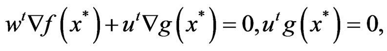
, such that

,.

Proof.

Since every efficient solution is a weak minimum, then by applying Theorem (2.2) of Weir and Mond [13] for x^*, we get, there exists such that

. (9)

, where.

REFERENCES

- B. D. Craven, “Control and Optimization,” Chapman and Hall, London, 1995.
- H. X. Phu, “Six Kind of Roughly Convex Functions,” Journal of Optimization Theory and Applications, Vol. 92, No. 2, 1997, pp. 357-375. doi:10.1023/A:1022611314673
- S. K. Mishra, S. Y. Wang and K. K. Lai, “Generalized Convexity and Vector Optimization, Nonconvex Optimization and Its Applications,” Springer-Verlag, Berlin, 2009.
- S. K. Mishra and G. Giorgi, “Invexity and Optimization, Nonconvex Optimization and Its Applications,” SpringerVerlag, Berlin, 2008.
- S. K. Suneja, S. Khurana and Vani, “Generalized Nonsmooth Invexity over Cones in Vector Optimization,” European Journal of Operational Research, Vol. 186, No. 1, 2008, pp. 28-40. doi:10.1016/j.ejor.2007.01.047
- S. Komlosi, T. Rapesak and S. Schaible, “Generalized Convexity,” Springer-Verlag, Berlin, 1994.
- M. A. Hanson, “On Sufficiency of the Kuhn-Tucker Conditions,” Journal of Mathematical Analysis and Applications, Vol. 80, No. 2, 1981, pp. 545-550. doi:10.1016/0022-247X(81)90123-2
- C. R. Bector, S. K. Sunela and C. Singh, “Generalization of Preinvex and B-vex Functions,” Journal of Optimization Theory and Applications, Vol. 76, No. 3, 1993, pp. 277-287. doi:10.1007/BF00939383
- T. Emam, “Roughly B-invex Programming Problems,” Calcolo, Vol. 48, No. 2, 2011, pp. 173-188. doi:10.1007/s10092-010-0034-5
- T. Morsy, “A Study on Generalized Convex Mathematical Programming Problems, Master Thesis, Faculty of Science,” Suez Canal University, Egypt, 2003.
- V. Chankong and Y. Y. Haimes, “Multiobjective Decision Making Theory and Methodology,” North-Holland, Amsterdam, 1983.
- M. S. Bazaraa and C. M. Shetty, “Nonlinear Programming-Theory and Algorithms,” John Wiley and Sons, Inc., New York, 1979.
- T. Weir and B. Mond, “Generalized Convexity and Duality in Multiple Objective Programming,” Bulletin of the Australian Mathematical Society, Vol. 39, No. 2, 1989, pp. 287-299. doi:10.1017/S000497270000277X