American Journal of Plant Sciences
Vol. 4 No. 7A1 (2013) , Article ID: 34550 , 10 pages DOI:10.4236/ajps.2013.47A1001
Calibrating Vegetation Cover and Grassland Pollen Assemblages in the Flint Hills of Kansas, USA
![]()
1Department of Geography, Kansas State University, Manhattan, USA; 2Institute of Ecology, Tallinn University, Tallinn, Estonia.
Email: julie.commerford@gmail.com
Copyright © 2013 Julie L. Commerford et al. This is an open access article distributed under the Creative Commons Attribution License, which permits unrestricted use, distribution, and reproduction in any medium, provided the original work is properly cited.
Received April 16th, 2013; revised May 18th, 2013; accepted June 15th, 2013
Keywords: Grassland; Pollen; Prairie; North America; Paleoecology
ABSTRACT
Grassland cover and composition respond to climate and have undoubtedly changed during the Holocene, but quantitative reconstructions from fossil pollen have been vague about spatial scale and taxon-specific cover. Here, we estimate the relevant source area of pollen for sedimentary basins approximately 50 m in radius, and we report pollen productivity estimates for 12 plant taxa in the tallgrass prairies of central North America. Both relevant source area of pollen and pollen productivity estimates were calculated via the Extended R-Value Model. To obtain these estimates, we collected and quantified the pollen found in surface sediment samples from 24 ponds across the study area. Vegetation was surveyed in the field in a 100 m radius around each pond, and vegetation maps from the Kansas Gap Analysis Project (GAP) were used to a radius of 2 km. Pollen fall speeds were calculated according to Stoke’s Law. Pollen assemblages from basins approximately 50 m in radius have a relevant source area of 1060 m in this grassland landscape. Pollen productivity estimates range from 0.02 to over 30 among the 12 taxa: Artemisia, Ambrosia, Asteraceae, Chenopodiaceae, Cornus, Fabaceae, Juniperus, Maclura, Poaceae, Populus, Quercus, and Salix. Woody taxa generally have higher pollen productivity than herbaceous taxa (except for Chenopodiaceae and Ambrosia).
1. Introduction
Reliable quantitative reconstructions of vegetation cover from pollen records remain a common goal of many paleoecologists and biogeographers [1]. Several factors complicate the relationship between vegetation cover and pollen produced by that vegetation and deposited in sediments, most notably differential pollen productivity among taxa and uncertainty about the spatial scale represented by the pollen assemblage. It has therefore been difficult to quantitatively reconstruct a landscape based on pollen percentages alone. Recent conceptual advances have allowed the calculation of pollen productivity estimates (PPEs) that account for differential pollen productivity among plant taxa [2,3]. However, calibration efforts are labor-intensive and the application of PPEs to landscape reconstruction is far from routine. In North America, hardly any PPE research has been done, with the exception of a few studies limited to forest ecosystems [4].
Quantitative modeling is a promising method for understanding land cover change in the paleorecord. There are two other ways to interpret pollen assemblages, each of which is useful for certain types of questions: 1) qualitative analyses, and 2) the modern analog technique. Qualitative analyses can help answer questions about landscape change based on interpretation of pollen percentages, especially using indicator taxa [5]. However, pollen percentages do not account for differences in pollen productivity among taxa. Modern analog techniques can statistically match pollen records from an unknown past landscape with those of a known modern landscape, and large datasets are now available for performing these analyses [6,7]. This technique is not effective for reconstructing land cover if an analog is not present [8], if detailed vegetation metadata are not available, or at fine spatial scales.
The alternative approach, quantitative modelling, produces estimates of landcover at relatively high taxonomic and spatial resolution that are relatively robust over time [2]. High-quality estimates of landcover change during the Holocene are especially important in grassland regions because of extreme climate variability in the past [9], and the potential for future climate change. Paleorecords, including pollen preserved in sediment, have been essential for determining the details of mid-Holocene climates and movement of the prairie-forest boundary in North America [10]. Past climate changes likely caused shifts in the composition of prairies and the proportion of bare ground, but these are currently unidentifiable in the North American pollen record.
Additionally, the spatial area represented by pollen in sediments is rarely investigated. Thus, pollen records can be presented without much information about the spatial scale they represent [11]. Generally speaking, small basins reflect local vegetation and large basins reflect regional vegetation [12,13]. All sedimentary basins have a relevant source area of pollen (RSAP) which is sometimes referred to as the “pollenshed” of the basin. The basic idea is that only the vegetation in a certain area surrounding each basin corresponds to the types and quantities of pollen deposited there. Correlations between plant abundance and pollen loading will improve as distance increases. At a certain distance, however, the correlation does not continue to improve, even with continued vegetation sampling to greater distances. The area surrounding the basin beyond which the correlation between pollen and vegetation does not improve is defined as the RSAP. RSAP can be calculated using the Extended RValue (ERV) models which are also used to calculate pollen productivity [2].
The Extended R-Value (ERV) models were proposed to overcome the difficulties associated with the use of pollen percentages and made it possible to estimate pollen productivity. These pollen productivity estimates are, for a given plant taxon, the slope of the linear relationship between pollen loading in absolute units and the vegetation composition with distance weighting [2]. PPEs are calculated relative to a reference taxon. The ERV models have been extensively used to calculate pollen productivity estimates in the upper Great Lakes region of the United States [14], southern Sweden [15], Denmark [16], Switzerland [17], Finland [18], Estonia [19], Norway [20], Scotland [21], and the United Kingdom [22]. Additionally, PPEs can be applied to landscape reconstruction models, such as the Landscape Reconstruction Algorithm (LRA) which uses PPEs to reconstruct vegetation cover based on pollen data [12,13].
In this study, we focused on the Flint Hills Tallgrass ecoregion, the largest remaining tract of tallgrass prairie vegetation in North America. We collected surface sediments from small ponds, acquired vegetation data, and conducted ERV modeling to achieve two primary aims: 1) to obtain a better understanding of the spatial relationship between pollen assemblages in small (50 m radius) ponds and vegetation cover on the landscape, through calculation of the RSAP, and 2) to provide pollen productivity estimates for 12 plant taxa common throughout the grasslands of central North America. First, we hypothesized that present-day pollen assemblages taken from sediment samples in ponds approximately 50 m in radius would be correlated with vegetation cover at the family-level to a distance of about 1000 m. This hypothesis is based on the results of studies from Europe that have examined mixed landscapes of forest and grassland [3]. Second, we hypothesized that common grassland plant taxa would differ in pollen productivity, with tree taxa being higher than Poaceae (the reference taxon), and most herbaceous taxa (except Chenopodiaceae and Ambrosia) being lower than Poaceae, because of their inherently different pollination habits. This hypothesis is based on the results of several PPE studies in Europe that have shown that tree taxa generally have higher PPEs than Poaceae, and most herbaceous taxa generally have lower PPEs than Poaceae [3].
2. Material and Methods
2.1. Study Area
The Flint Hills Tallgrass Ecoregion is located in eastern Kansas, USA (Figure 1). The Flint Hills comprise alternating layers of limestone and other sedimentary rock deposited during the Permian in a shallow inland sea. Modern climate in the Flint Hills region exhibits high seasonal and interannual variability, with high temperatures ranging from 25˚C to 38˚C in the summer and low temperatures ranging from −12˚C to −6˚C in the winter at the Tallgrass Prairie Preserve (US National Park Service, 2010), close to the geographic center of the ecoregion. Average annual precipitation generally averages 75 cm (US National Park Service, 2010). In the summer, severe thunderstorms with heavy downpours and hail are common. Winter snowfall events occur, especially in the northern part of the Flint Hills.
Tallgrass prairie dominates the vegetative cover of the Flint Hills (Figure 1). More than 98% of tallgrass prairie cover has been lost in the past 200 years due to its widespread conversion to row-crop agriculture [23]. The Flint Hills contains the largest remaining tract of tallgrass prairie on the continent because the shallow, rocky soils are unsuitable for tillage and are instead grazed by cattle. Tallgrass vegetation is characterized by an abundance of warm-season grasses such as big bluestem (Andropogon gerardii) and Indian grass (Sorghastrum nutans). There are several common forbs including various sunflower, goldenrod, sage, and ragweed species in the family Asteraceae. Eastern red cedar (Juniperus virginiana), burr oak (Quercus macrocarpa), and cottonwood (Populus deltoides) are some of the tree species present. Woody cover has been increasing in the region since the beginning of the 20th century [24].
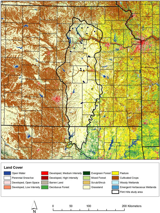
Figure 1. Location of 24 ponds for sediment acquisition in the Flint Hills study area with land cover types from US National Land Cover Data set (2001). Flint Hills boundary follows US Environmental Protection Agency.
We selected our pollen sampling sites to be small ponds that were distributed as randomly as possible while still covering a large portion of the study area (Figure 1). This has been shown to be an effective sample design for calculating PPEs [21]. Vegetation cover varied on a siteto-site basis for each of the ponds sampled. The majority of the sites included woody components at the edge of the pond, with grasses and herbs beyond the woody areas. Some sites contained no woody species within 100 m radius of the pond edge, and some were dominated by woody species within 100 m.
2.2. Pollen Data Acquisition
Surface sediment samples were acquired from 24 ponds across the Flint Hills of Kansas. Each pond was less than 10 hectares in size, and averaged 50 m in radius. Pollen was isolated from bulk sediment using a series of chemical digestions including acetolysis and other standard techniques [25]. Pollen grains for each sample were identified visually in a light microscope at 400× resolution to a sum of at least 300 grains. A total of 75 arboreal and herbaceous upland pollen taxa were found in the pollen assemblages: 38 arboreal and 37 herbaceous pollen types. Pollen percentages are reported in [26].
2.3. Vegetation Data Acquisition
Because the ERV model requires distance-weighted vegetation data as an input file, a nested vegetation survey method was used, in which vegetation closest to the pond (0 - 100 m) was surveyed in the finest detail, with less detail at greater distances (100 - 2000 m). Vegetation was surveyed at each site along four predetermined transects —one oriented along each cardinal direction—stretching from the edge of the pond to a distance of 100 m from the pond. For each transect, percent cover of the vegetation was estimated to the family or genus level at 10 m increments, with one plot at each distance increment along each transect. We used a modified Daubenmire method for estimating vegetation cover where the quadrat size was 1 m2. In addition to the quadrat data, we recorded the location of trees and patches of woody shrubs, since trees and shrubs were often missed in the vegetation surveys, yet still contribute to the pollen assemblage. From 0 - 10 meters in radius from the edge of each pond, we recorded the location of each individual tree and shrub, and identified it to the genus level. From 10 - 100 meters in radius, we marked the location of all patches of trees and shrubs and identified the genera present in the patch.
In addition to the field surveys, a state-wide vegetation map of Kansas from the Kansas Gap Analysis Project (GAP) (http://kars.ku.edu/products/maps/kansas-vegetation-map-aka-kansas-gap-map/) was used. This map was produced by the Kansas Applied Remote Sensing Program and is based on multi-seasonal LANDSAT imagery that was acquired in 1993. It has a cell size of 30 meters by 30 meters. This data set was selected because of its high taxonomic resolution: 43 land cover classes, most of which pertain to natural land cover rather than human-induced land cover.
In GIS, the digitized field maps were overlain on the GAP map, and buffers were constructed every 10 m from the shore of each pond to 2000 m. Areas were calculated for each vegetation category within each 10 meter ring. For woody categories, areas were divided evenly among the taxa indicated for that category. For example, 1000 m2 of Salix-Populus woodland became 500 m2 Salix and 500 m2 Populus. For all categories that are grassland or some variation of grassland, we applied the field data for percent cover of each family. Because the grassland taxa are not represented in the GAP maps in the same detail as the tree taxa, this step further defines the grassland category. At each site, we multiplied the total area of grassland by the percent cover of each family at that distance. For example, we multiplied the total area of grassland within the 0 - 10 meter ring by the percentages from the 10-meter field quadrats at each site. This procedure was followed to 100 meters. Because the field vegetation surveys extended only to 100 m, we selected four quadrats from that overall site and multiplied those percentages by the grassland category for distances greater than 100 m. This procedure was followed to a 2000 m radius, which is the largest distance likely to be contributing local pollen to the pond, based on other studies in Europe that have estimated this distance for similar size basins [3].
2.4. Pollen Fall Speed
The speed at which pollen falls is dependent on the size and shape of the pollen, and thus it is unique to a pollen type [27]. The fall speeds for Juniperus, Poaceae, Quercus, and Salix, were calculated in previous studies [28, 29]. For Ambrosia, Artemisia, Asteraceae, Chenopodiaceae, Cornus, Fabaceae, Maclura, and Populus, fall speeds had not been previously calculated. These fall speeds were calculated according to Stoke’s Law [27], and following Sugita et al. (1999) (Table 1).
2.5. ERV Modeling
Pollen productivity estimates (PPEs) and Relevant Source Area of Pollen (RSAP) were calculated with a modified Extended R-Value (ERV) model [2]. This pollen-vegetation model was written by Shinya Sugita (Tallinn University, Estonia) and has been extensively tested in Europe. The ERV Model describes the pollen-vegetation relationship as a linear function:
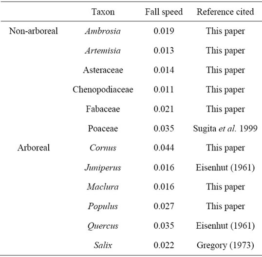
Table 1. Fall speed of pollen grains for selected taxa.
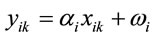 (1)
(1)
whereyik = pollen loading of species i at site k xik = vegetation abundance of species i at site k
αi = pollen productivity of species i
ωi = background pollen loading for species i Three sets of files are required for ERV modeling: distance weighted vegetation abundance for each site, pollen counts for each site, and fall speed of each taxon. The vegetation abundance set of files contains one spreadsheet for each of the 24 sites, with distance increments set at 10 meters. The pollen counts file contains one sheet with the total number of pollen grains of each taxon at each site. The fall speed file contains one sheet listing each plant taxon and its associated fall speed.
In addition to these files, ERV models require the wind speed, the basin radius, and the desired pollen dispersal model. We entered a wind speed of 5 m/s, and a basin radius of 50 m, which is the average radius of all 24 ponds. For the pollen dispersal model, we used the Ring Source-Lake/Pond Model. Furthermore, an estimate of RSAP can be acquired if a moving-window size is specified. This spatial moving-window value affects the shape of the curve of the likelihood function score used to estimate RSAP. With this method, the RSAP is estimated to be the distance at which the likelihood function score approaches an asymptote, or when the difference between values becomes 0.1 or lower for a distance of 50 m. We specified a moving window of 300 m. Typical values fall between 200 m and 400 m [30].
There are three submodels to ERV, which vary according to how they define background pollen. Background pollen is the pollen coming from beyond the RSAP. Submodel 1 describes background pollen relative to the total pollen loading for each taxon. Submodel 2 describes background pollen as being the ratio of the pollen coming from beyond the distance of the vegetation data used in the analysis, to the total vegetation abundance within the area of the vegetation used in the analysis. In submodel 3, the background pollen simply represents the pollen coming from outside the area of the vegetation data used for the analysis. All three submodels were tested in order to obtain the best and most reliable estimate of pollen productivity for each taxon.
3. Results
The RSAP estimate for the 24 ponds in this study varies between 1050 m and 1060 m, depending on which submodel is used (Figure 2). Submodel 1 produced an RSAP of 1050 m, and Submodel 3 produced an RSAP of 1060 m. Submodel 2 was unable to produce an RSAP. The RSAP values of 1050 m and 1060 m suggest that the relationship between the pollen assemblage and the vegetation cover does not improve past 1050 - 1060 m. The jagged shape of the curve of the log-likelihood values for Submodel 1 suggests that it may not be suitable for this environment (Figure 2). However, it is still useful to compare the results from both submodels in order to fully understand the estimates that they provide regarding the pollen-vegetation relationship. Since Sub-model 1 assumes that background pollen loading in the pollen proportions is a species-specific constant among sites, settings with large site-to-site variation in background pollen would not be a proper fit for Submodel 1. Log-likelihood values for Submodel 3 display a smooth curve, and thus Submodel 3 is a better fit for the Flint Hills study area.
The submodels of ERV attempt to find the best linear relationship between the pollen and the vegetation. Scatterplots of the pollen-vegetation relationship show that there is a relationship between the pollen and vegetation data (Figure 3). While these plots are helpful for visualizing the pollen-vegetation relationships, PPEs are cal-

Figure 2. Log-likelihood plots for ERV Submodel 1, 2, and 3. There are several possible reasons for this shape, including the structure of the semi-open landscape in the Flint Hills, and systematic changes in vegetation composition with increasing distance from the pond edge.
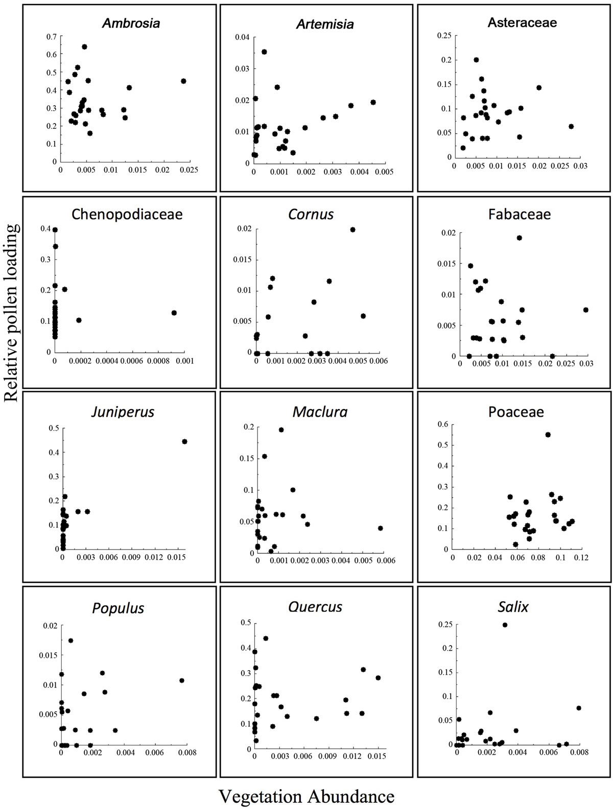
Figure 3. ERV Plots from submodel 3. Relative pollen loading versus absolute vegetation cover. Each dot represents one site.
culated separately by the model, so an r-value of correlation is not necessary.
Pollen productivity estimates for each of the 12 taxa were produced using ERV Submodel 1 and Submodel 3 (Table 2, Figure 4). Because the best estimate of PPE is obtained at the distance of the RSAP and beyond, the average and standard deviation of all PPE for each taxa from a distance of the RSAP to 2000 m was calculated. This is used to smooth out any slight variation in PPE beyond the RSAP. PPEs were calculated relative to Poaceae because of its intermediate relative pollen productivity, and thus Poaceae has a PPE of 1.0 for both submodels. Juniperus had the highest PPE using Submodel 3, and Chenopodiaceae had the highest PPE using Submodel 1 and Fabaceae had the lowest PPE with both submodels (Table 2).
4. Discussion
4.1. Relevant Source Area of Pollen
Previous studies have estimated RSAP to be between 300
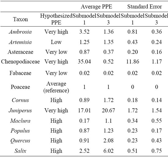
Table 2. Hypothesized PPE, calculated average PPE, and standard error of PPE for all selected taxa from distance of RSAP to maximum survey distance.
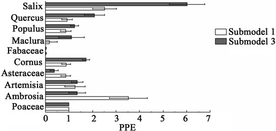
Figure 4. PPEs with standard errors for all taxa, excluding Chenopodiaceae and Juniperus (for visualization purposes).
and 1700 m for small lakes approximately 100 m in radius [2,16,28]. The RSAP of 1060 m for small lakes in the Flint Hills falls near the middle of this range, and it also supports our first hypothesis, in which we predicted RSAP to be approximately 1000 m. While basin size clearly has an effect on RSAP, because small basins serve as catchments for pollen originating from relatively local areas surrounding the ponds, landscape openness and vegetation patch sizes also have been shown to have an effect on RSAP [28,31]. In addition, Sugita et al. (1999) examined RSAP for simulated open and semi-open landscapes in southern Sweden, and noted that ponds in open and semi-open landscapes had a RSAP of 800 to 1000 m. In closed forests of northern Michigan, Sugita (1994) simulated the RSAP for small ponds to be 300 m. The drastic difference in RSAP between the open and semiopen landscape versus the closed landscape was predicted to be due to the distribution of the vegetation on the landscape. In the closed landscape, vegetation patches were much more frequent, and therefore the distance required to achieve constant background pollen among sites was much smaller.
The landcover of the Flint Hills of North America resembles the southern Sweden landscape in several aspects: there is a matrix of herbaceous taxa with scattered tree taxa punctuating this matrix. Overall, the woody cover is less than 30% for the Flint Hills, which would define it as a grassland by most assessments [32]. The RSAP for small ponds in North American tallgrass prairie is 1060 m, which is similar to the RSAP for semiopen landscapes in Sweden. There are several possible reasons for this similarity. First, tree taxa at the Flint Hills sites were usually present within the first 10 m from the edge of the pond, with scattered clumps beyond 10 m. This vegetation distribution would probably lead to an RSAP that most closely aligns with the semi-open landscape. Although the grasslands of the Flint Hills appear to be very open, the presence of trees directly adjacent to the sampled ponds could cause the landscape to behave more like a semi-open landscape than an open landscape. Second, the presence of rare taxa in a landscape leads to an increase in RSAP [31]. In the Flint Hills, the tree taxa would be considered rare taxa, since herbaceous taxa typically comprise the majority of the vegetation cover on the landscape. These taxa make the landscape less homogenous, causing the RSAP to be reached at a greater distance than if there were no rare taxa present.
4.2. Pollen Productivity Estimates
The PPE values for each of the 12 taxa represent the productivity of each taxa in reference to Poaceae (1.0). With the results from submodel 3, most tree taxa seem to have higher PPE values than Poaceae, which has also been a trend in previous studies [3]. The herbaceous taxa—Ambrosia, Artemisia, Asteraceae, Chenopodiaceae, Fabaceae, and Poaceae—have lower PPEs than most of the woody taxa (except Maclura and Populus). Even though some of the herbaceous taxa are wind-pollinated, they are much smaller organisms than trees and thus produce smaller amounts of pollen on average. Additionally, herbaceous taxa that are insect-pollinated such as Fabaceae have very low PPEs, consistent with their pollination biology [33]. This finding is consistent with our second hypothesis, which predicted that herbaceous taxa would have generally lower PPEs than most of the woody taxa.
Chenopodiaceae is an outlier among the other taxa, because it has a very high PPE (35.04) with submodel 1, and a very low PPE (0.52) with submodel 3. Neither of these values seems to be a good indicator of the actual PPE for Chenopodiaceae, for several reasons. First, Chenopodiaceae should have a high PPE in theory, because it had a very high presence in the pollen assemblage, but very low presence in the vegetation surveys. Since the standard error was also high (11.86) with submodel 1, neither submodel seems to produce an accurate value. Second, in order to obtain accurate PPEs, it is recommended that the selected taxa be present in both the pollen and vegetation record of at least half of the sites [3]. In this study, Chenopodiaceae was present in the pollen for at least half of the sites, but was not present in the vegetation survey for half of the sites.
The problem that arises with Chenopodiaceae may not be unique to this taxon, but is likely due to its rare presence on the landscape, coupled with its strong presence in the pollen data. If a taxon is very rare on the landscape but shows a strong presence in the pollen data, it would theoretically have a high PPE, but there would be insufficient site-to-site data to mathematically calculate this PPE with the ERV Model. This situation occurred with Chenopodiaceae. Other taxa, such as Juniperus, also had a strong presence in the pollen data, but had an average presence in the vegetation surveys at the sites, and were present at almost all of the sites. This presence in the vegetation data allowed for a more accurate calculation of PPE with a lower standard error for Juniperus.
These PPEs are the first reported for North American herbaceous taxa, and it is useful to compare them with PPEs calculated for the same pollen types in Europe (Broström et al., 2008). Variations between North American and European PPEs might be due to the same pollen type consisting of different plant species, a situation that also occurs within regions of North America [34]. For example, most of the Quercus present in this study was Quercus macrocarpa, a species that is common in riparian areas in the Flint Hills. The Quercus taxon in European studies was composed of Quercus robur [15]. In west central Sweden, it has been observed that PPEs may vary among species, and therefore taxa composed of different species might not be directly comparable [35]. This distinction supports the necessity of obtaining PPEs for a particular study area before attempting to use the PPEs for vegetation reconstruction, or at least the same continent, since PPEs might not be directly transferrable from one region to another.
Future research can examine the composition of the background pollen in this region by examining surface samples from larger lakes [12]. Once background pollen can be quantified for the region, it will be possible to apply the Landscape Reconstruction Algorithm to grassland systems of North America [36]. The timing of changes in the prairie-forest ecotone in North America has recently been shown to be much more rapid than previously thought [37]. Our results combined with more regional assessments will enable finer-scale reconstructions at this boundary (less than the 11 km by 11 km window around surface sample sites) and provide greater taxonomic resolution relevant for ecologists and managers. The pollen productivity estimates obtained in this study are the first PPEs to be obtained for any grassland region in North America. The differences reported here in PPEs among continents (Europe and North America) demonstrate the value of obtaining PPEs that are directly applicable to the region that one is studying. The PPEs reported here can be used for landscape reconstruction, and they add to a growing understanding of the quantitative relationship between vegetation cover and pollen assemblages.
5. Acknowledgements
We gratefully acknowledge all of the landowners and ranchers in the Flint Hills who granted access to their ponds and grasslands. We thank N. Brenner and T. Graver for fieldwork assistance, V. Stefanova for counting the pollen, and the University of Minnesota Limnological Research Center for pollen preparation. We thank J.M.S. Hutchinson and D. Goodin for helpful comments. The research was supported by grant BCS-0821959 from the National Science Foundation of the United States of America.
REFERENCES
- H. Seppä and K. D. Bennett, “Quaternary Pollen Analysis: Recent Progress in Palaeoecology and Palaeoclimatology,” Progress in Physical Geography, Vol. 27, No. 4, 2003, pp. 548-579. doi:10.1191/0309133303pp394oa
- S. Sugita, “Pollen Representation of Vegetation in Quaternary Sediments: Theory and Method in Patchy Vegetation,” Journal of Ecology, Vol. 82, No. 4, 1994, pp. 881- 897. doi:10.2307/2261452
- A. Broström, et al., “Pollen Productivity Estimates of Key European Plant Taxa for Quantitative Reconstruction of Past Vegetation: A Review,” Vegetation History and Archaeobotany, Vol. 17, No. 5, 2008, pp. 461-478. doi:10.1007/s00334-008-0148-8
- S. Sugita, et al., “Testing the Landscape Reconstruction Algorithm for Spatially Explicit Reconstruction of Vegetation in Northern Michigan and Wisconsin,” Quaternary Research, Vol. 74, No. 2, 2010, pp. 289-300. doi:10.1016/j.yqres.2010.07.008
- V. Zernitskaya and N. Mikhailov, “Evidence of Early Farm- ing in the Holocene Pollen Spectra of Belarus,” Quarternary International, Vol. 203, No. 1-2, 2009, pp. 91-104. doi:10.1016/j.quaint.2008.04.014
- J. Whitmore, et al., “Modern Pollen Data from North American and Greenland for Multi-Scale Paleoenvironmental Applications,” Quaternary Science Reviews, Vol. 24, No. 16-17, 2005, pp. 1828-1848. doi:10.1016/j.quascirev.2005.03.005
- Y. Li, et al., “A Transfer-Function Model Developed from an Extensive Surface-Pollen Data Set in Northern China and Its Potential for Paleoclimate Reconstructions,” The Holocene, Vol. 17, No. 7, 2007, pp. 897-905. doi:10.1177/0959683607082404
- S. T. Jackson and J. W. Williams, “Modern Analogs in Quaternary Paleoecology: Here Today, Gone Yesterday, Gone Tomorrow?” Annual Review of Earth and Planetary Sciences, Vol. 32, 2004, pp. 495-537. doi:10.1146/annurev.earth.32.101802.120435
- A. Michels, et al., “Multidecadal to Millennial-Scale Shifts in Drought Conditions on the Canadian Prairies over the Past Six Millennia: Implications for Future Drought Assessment,” Global Change Biology, Vol. 13, No. 7, 2007, pp. 1295-1307. doi:10.1111/j.1365-2486.2007.01367.x
- J. W. Williams, et al., “Rapid, Time-Transgressive, and Variable Responses to Early Holocene Midcontinental Drying in North America,” Geology, Vol. 38, No. 2, 2010, pp. 135-138. doi:10.1130/G30413.1
- E. A. C. Rushton, S. E. Metcalfe and B. S. Whitney, “A Late-Holocene Vegetation History from the Maya Lowlands, Lamanai, Northern Belize,” Holocene, Vol. 23, No. 4, 2013, pp. 485-493. doi:10.1177/0959683612465449
- S. Sugita, “Theory of Quantitative Reconstruction of Vege- tation I: Pollen from Large Sites Reveals Regional Vegetation Composition,” Holocene, Vol. 17, No. 2, 2007, pp. 229-241. doi:10.1177/0959683607075837
- S. Sugita, “Theory of Quantitative Reconstruction of Vegetation II: All You Need Is Love,” Holocene, Vol. 17, No. 2, 2007, pp. 243-257. doi:10.1177/0959683607075838
- S. Sugita, T. Parshall and R. Calcote, “Detecting Differences in Vegetation among Paired Sites Using Pollen Records,” Holocene, Vol. 16, No, 8, 2006, pp. 1123-1135. doi:10.1177/0959683606069406
- A. Broström, S. Sugita and M. J. Gaillard, “Pollen Productivity Estimates for the Reconstruction of Past Vegetation Cover in the Cultural Landscape of Southern Sweden,” Holocene, Vol. 14, No. 3, 2004, pp. 368-381. doi:10.1191/0959683604hl713rp
- A. B. Nielsen and S. Sugita, “Estimating Relevant Source Area of Pollen for Small Danish Lakes around AD 1800,” Holocene, Vol. 15, No. 7, 2005, pp. 1006-1020. doi:10.1191/0959683605hl874ra
- W. Soepboer, et al., “Pollen Productivity Estimates for Quantitative Reconstruction of Vegetation Cover on the Swiss Plateau,” Holocene, Vol. 17, No. 1, 2007, pp. 65- 77. doi:10.1177/0959683607073279
- S. Sugita, S. Hicks and H. Sormunen, “Absolute Pollen Pro- ductivity and Pollen-Vegetation Relationships in Northern Finland,” Journal of Quaternary Science, Vol. 25, No. 5, 2010, pp. 724-736. doi:10.1002/jqs.1349
- A. Poska, et al., “Relative Pollen Productivity Estimates of Major Anemophilous Taxa and Relevant Source Area of Pollen in a Cultural Landscape of the Hemi-Boreal Forest Zone (Estonia),” Review of Palaeobotany and Palynology, Vol. 167, No. 1-2, 2011, pp. 30-39. doi:10.1016/j.revpalbo.2011.07.001
- K. L. Hjelle and S. Sugita, “Estimating Pollen Productivity and Relevant Source Area of Pollen Using Lake Sediments in Norway: How Does Lake Size Variation Affect the Estimates?” Holocene, Vol. 22, No. 3, 2012, pp. 313- 324. doi:10.1177/0959683611423690
- C. L. Twiddle, et al., “Pollen Productivity Estimates for a Pine Woodland in Eastern Scotland: The Influence of Sampling Design and Vegetation Patterning,” Review of Palaeobotany and Palynology, Vol. 174, 2012, pp. 67-78. doi:10.1016/j.revpalbo.2011.12.006
- M. J. Bunting, et al., “Estimates of ‘Relative Pollen Productivity’ and ‘Relevant Source Area of Pollen’ for Major Tree Taxa in Two Norfolk (UK) Woodlands,” Holocene, Vol. 15, No. 3, 2000, pp. 459-465. doi:10.1191/0959683605hl821rr
- F. B. Samson, F. L. Knopf and W. R. Ostlie, “Great Plains Ecosystems: Past, Present, and Future,” Wildlife Society Bulletin, Vol. 32, No. 1, 2004, pp. 6-15. doi:10.2193/0091-7648(2004)32[6:GPEPPA]2.0.CO;2
- J. M. Briggs, et al., “An Ecosystem in Transition. Causes and Consequences of the Conversion of Mesic Grassland to Shrubland,” Bioscience, Vol. 55, No. 3, 2005, pp. 243- 254. doi:10.1641/0006-3568(2005)055[0243:AEITCA]2.0.CO;2
- K. Faegri, P. E. Kaland and K. Kzywinski, “Textbook of Pol- len Analysis,” 4th Edition, John Wiley, Hoboken, 1989, p. 328.
- K. K. McLauchlan, J. L. Commerford and C. J. Morris, “Tallgrass Prairie Pollen Assemblages in Mid-Continental North America,” Vegetation History and Archaeobotany, Vol. 22, No. 3, 2013, pp. 171-183. doi:10.1007/s00334-012-0369-8
- P. H. Gregory, “The Microbiology of the Atmosphere,” Leonard Hill, Aylesbury, 1973.
- S. Sugita, M.-J. Gaillard and A. Brostrom, “Landscape Openness and Pollen Records: A Simulation Approach,” Holocene, Vol. 9, No. 4, 1999, pp. 409-421. doi:10.1191/095968399666429937
- G. Eisenhut, “Investigations on the Morphology and Ecology of Pollen Grains of Native and Introduced Forest Trees,” Paul Parey, Hamburg, 1961.
- M.-J. Gaillard, et al., “The Use of Modelling and Simulation Approach in Reconstructing Past Landscapes from Fossil Pollen Data: A Review and Results from the POLLANDCAL Network,” Vegetation History and Archaeobotany, Vol. 17, No. 5, 2008, pp. 419-443. doi:10.1007/s00334-008-0169-3
- M. J. Bunting, et al., “Vegetation Structure and Pollen Source Area,” Holocene, Vol. 14, No. 5, 2004, pp. 651- 660. doi:10.1191/0959683604hl744rp
- R. C. Anderson, J. S. Fralish and J. M. Baskin, “Savannas, Barrens, and Rock Outcrop Plant Communities of North America,” Cambridge University Press, Cambridge, 1999.
- L. A. Real, “Pollination Biology,” Academic Press, Inc., Orlando, 1983.
- J. W. Williams and B. Shuman, “Obtaining Accurate and Precise Environmental Reconstructions from the Modern Analog Technique and North American Surface Pollen Dataset,” Quaternary Science Reviews, Vol. 27, No. 7-8, 2008, pp. 669-687. doi:10.1016/j.quascirev.2008.01.004
- H. von Stedingk, R. M. Fyfe and A. Allard, “Pollen Productivity Estimates from the Forest-Tundra Ecotone in West-Central Sweden: Implications for Vegetation Reconstruction at the Limits of the Boreal Forest,” Holocene, Vol. 18, No. 2, 2008, pp. 323-332. doi:10.1177/0959683607086769
- S. Hellman, et al., “The Reveals Model, a New Tool to Estimate Past Regional Plant Abundance from Pollen Data in Large Lakes: Validation in Southern Sweden,” Journal of Quaternary Science, Vol. 23, No. 1, 2008, pp. 21-42. doi:10.1002/jqs.1126
- J. W. Williams, B. Shuman and P. J. Bartlein, “Rapid Responses of the Prairie-Forest Ecotone to Early Holocene Aridity in Mid-Continental North America,” Global and Planetary Change, Vol. 66, No. 3/4, 2009, pp. 195-207. doi:10.1016/j.gloplacha.2008.10.012