Advances in Computed Tomography
Vol.3 No.1(2014), Article ID:44326,10 pages DOI:10.4236/act.2014.31001
Optimization of Contrast Material Dose for Abdominal Multi-Detector Row CT: Predicting Patient Lean Body Weight by Using Preliminary Transverse CT Images
Antonino Guerrisi1, Daniele Marin2, Huiman Barnhart3, Lisa Ho2, Thomas L. Toth4, Carlo Catalano1, Rendon C. Nelson2
1Department Department of Radiological Sciences, University of Rome Sapienza, Rome, Italy
2Department of Radiology, Duke University Medical Center, Durham, USA
3Department of Biostatistics and Bioinformatics Duke Clinical Research Institute, Durham, USA
4G.E. Medical Systems, Milwaukee, USA
Email: antonioguerrisi@msn.com
Copyright © 2014 by authors and Scientific Research Publishing Inc.
This work is licensed under the Creative Commons Attribution International License (CC BY).
http://creativecommons.org/licenses/by/4.0/


Received 24 December 2013; revised 25 January 2014; accepted 1 February 2014
ABSTRACT
Estimated LBW could be used to determine the contrast material dose and rate during MDCT. The aim of this study is to test the accuracy of a technique for estimation of lean body weight (LBW) from a single multi-detector row computed tomographic (MDCT) abdominal image, using a bioelectrical body composition analyzer scale as the reference standard. CT images of 21 patients with previously measured LBW (mLBW) were processed using computer-assisted, vendor-specific software (Advantage Windows 4.2; GE Healthcare, Inc). For each transverse image, a fat-fraction was automatically measured as the number of fat pixels (−200 to −50 HU) divided by the total number of pixels having an attenuation value ≥−200 HU. Estimated LBW (eLBW) of five single contiguous sections was calculated in each of three abdominal regions (upper abdomen, mid abdomen and pelvis) by multiplying TBW by (1 – fat-fraction). Bland-Altman plot with limits of agreement was used to assess agreement between mLBW and eLBW. The mean mLBW for all patients was 56 kg (range, 39 - 75 kg). Mean differences and limits of agreement between mLBW and eLBW measurements for the upper abdomen, mid abdomen and pelvis reported were −8.9 kg (−25.6 kg, +7.5 kg), −10.6 kg (−27.7 kg, +6.4 kg), and +0.5 kg (−12.8 kg, +13.8 kg) respectively. eLBW deriving directly from a transverse CT image of the pelvis can accurately predict mLBW.
Keywords:Lean Body Weight; Multi-Detector CT; Contrast Dose

1. Introduction
The dose and rate of iodinated contrast medium used during abdominal multi-detector row computed tomography (MDCT) need to be tailored to individual patients in order to obtain uniform vascular and parenchymal enhancement among patients with different body sizes. Although using a fixed dose of contrast medium has been shown to be easy to implement and is generally effective, it can result in an underor over-dosage of contrast medium in many patients [1] [2] . Preliminary evidence suggests that determining the dose and injection rate of contrast material administration based on the patient’s lean body weight (LBW) may improve patient-to-patient enhancement variability during vascular and abdominal MDCT [2] -[5] . In fact, contrast injection protocols based on LBW reduce the contribution of highly variable but poorly perfused adipose tissue to the dose estimate. This approach is particularly beneficial in large patients, where unnecessarily high doses of contrast material may be administered based on the patient total body weight, increasing the risk of side effects from contrast material as well as costs [2] . A variety of methods have been proposed for determining a patient’s LBW [6] [7] ; however, most of them are either subject to measurement error [7] [8] or are not practical for daily clinical use [9] -[11] . Foot-to-foot bioelectrical impedance analysis (FF-BIA) is one of the most accurate and easiest methods to measure LBW, however, it requires the use of a body composition weight analyzer scale and strict pretest instructions for the patient, which may limit its use in a busy radiology practice [12] [13] . Although CT has been shown to accurately measure percent body fat (PBF) and has been used to analyze the human body composition [14] -[16] , to our knowledge, no previous study has investigated the feasibility of using MDCT to estimate patient’s LBW. Advancements in computer software have made it possible to extract quantitative data from two-dimensional CT images in the clinical setting in an automated fashion [17] , thereby creating the possibility of accurate estimation of LBW for adjusting the contrast material dose and rate.
The purpose of this study was to determine whether a computer generated patient fat-fraction, deriving from a single, preliminary transverse MDCT image can be used to estimate LBW, and to determine the accuracy of this method when compared with FF-BIA.
2. Material and Methods
This Health Insurance Portability and Accountability Act-compliant retrospective study was approved by the local Institutional Review Board with a waiver of written informed consent.
2.1. Patient Population
Twenty-one consecutive patients who underwent contrast-enhanced MDCT of the abdomen and pelvis for clinically indicated reasons were retrospectively selected.General indications for CT imaging included the following: cancer (n = 16), abdominal pain (n = 1), hematuria (n = 1), diverticulitis (n = 1), abdominal abscess (n = 1), and suspected abdominal mass (n = 1). Before the diagnostic CT, the patient’s LBW (mLBW) was measured using the FF-BIA method. In addition, height, total body weight (TBW), and body mass index (BMI) (defined as the patient’s TBWin kilograms divided by height in squared meters [kg/m2]) were recorded for each patient (Table 1).
Exclusion criteria for this retrospective study included patient’s use of diuretics or pacemaker, both of which can interfere with FF-BIA measurements. No patient was excluded for the above mentioned reasons.
2.2. CT Technique
Multiphasic CT was performed with a 16-section MDCT scanner (Light Speed 16; GE Healthcare, Inc., Waukesha, WI) using a standard (Table 2).
All image data were sent electronically to a picture archiving and communication system (PACS) workstation (Centricity 1.0 or 2.1; GE Healthcare, Inc.) for interpretation. Patients were positioned supine with feet first on the scanning table.
After acquisition of anteroposterior and mediolateral digital scout radiographs, patients were scanned craniocaudally after intravenous (IV) contrast material administration during the hepatic venous phase.
The contrast material used for all patients was iopamidol (Isovue 370; Bracco Diagnostics, Princeton, NJ), with an iodine concentration of 370 mg/mL.
All patients received a contrast material dose based on lean body weight using a previously described method

Table 1. Demographics and clicical findings of the study population.
Table 2. Multi-Detector Row CT scanning parameter and reconstruction algorithm.
[2] . Patients received an average contrast media dose of 135 mL injected at 4.3 mL/sec.
2.3. Calculation of Percent Body Fat (PBF) and Measured LBW (mLBW)
For all 21 patients, percent body fat (PBF) was determined using a body composition and analyzer scale (Tanita Body Fat-300A; Tanita Corporation of America, Inc., Arlington Heights, IL). mLBW was calculated with the following formula: mLBW = TBW * (1 − PBF), where TBW is the patient’s total body weight and PBF is percent of body fat. In addition, before performing FF-BIA, the research assistant questioned the subjects as to their usual level of physical activity and this information was entered into the scales for a correct assessment of mLBW. The height of each subject was measured using a portable stadiometer and weight was measured using the analyzer scale. Height, weight, and age were then entered into the scale.
To ensure normal hydration status for FF-BIA testing, subjects were asked to adhere to the following pretest requirements: 1) no eating or drinking for four hours before testing; 2) no caffeine or alcohol consumption within 12 hours of the test; and 3) no vigorous exercise within 12 hours of the test [11] . Subjects were measured standing erect with bare feet on the analyzer footpads. The FF-BIA was conducted as follows: first, an electrical impulse was sent through the plantar surface of one foot, conducted up one legand down the other, and then received through the plantar surface of the contralateral foot.
2.4. Calculation of Patient Fat Fraction (PBF) and Estimated LBW (eLBW)
For the estimation of the LBW using CT images, three standardized body regions—defined as the upper abdomen, mid abdomen, and pelvis—were identified by two abdominal radiologists (A.G., D.M.) in consensus. To improve consistency in the identification of the three body regions, we used well-defined anatomical landmarks that could be readily recognizable from the scout radiograph. This included the L1 lumbar vertebral body for the upper abdomen, the L5 lumbar vertebral body for the mid abdomen, and the acetabular roof for the pelvis. To investigate possible significant differences due to slice selection, five contiguous 5-mm transverse CT images acquired during the abdominal venous phase were analyzed for each of the three anatomical locations identified on the anteroposterior digital scout radiograph. The commercially available software three-dimensional (3D) cube tool (Vox Tool, version 6.12.3) was used to calculate the patient fat-fractions for each transverse CT image (Figure 1).
This tool applies different attenuation thresholds to a selected image accurately differentiating fat pixels (attenuation values ranging between −200 HU and −50 HU) from tissue pixels (attenuation values ranging greater than −50 HU). After pixel-by-pixel segmentation of the cross sectional area of the CT image, the patient fat-fraction for each image was calculated by the following equation: [total fat pixels area/(total fat pixels area + total tissue pixels area)] × 100 (figures 2-4). The eLBW of the five CT images for each of the three body regions was then calculated using the following equation: patient TBW * (1-fat_fraction) (figure 5).
2.5. Statistical Analysis
Analyses were performed to determine the reproducibility of eLBW across the five images within the specific region, the agreement between mLBW and eLBW based on one image, and the factors that may impact the agreement between mLBW and eLBE. Intraclass correlation coefficient (ICC) and repeatability coefficient (RC) were used to assess the reproducibility ofeLBW measurements for the five transverse CT images at each of the
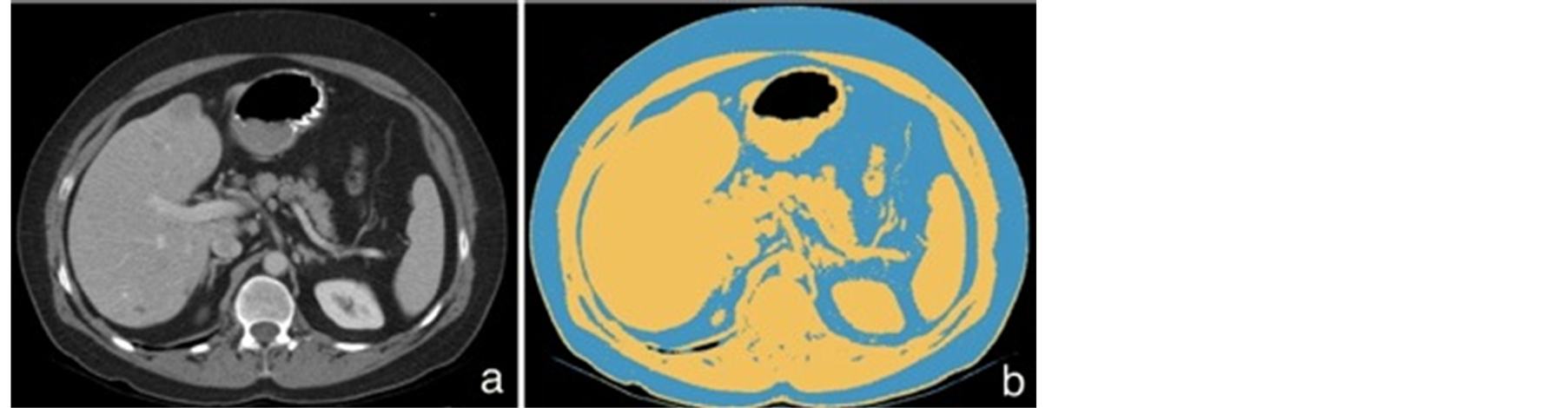
Figure 1. Transverse CT image in the upper abdomen (a) and automated segmentation of total adipose tissue of the same image (b). The yellow color represents pixels from −50 to 1000 HU, the blue color, pixels from −200 to −50 HU (b).
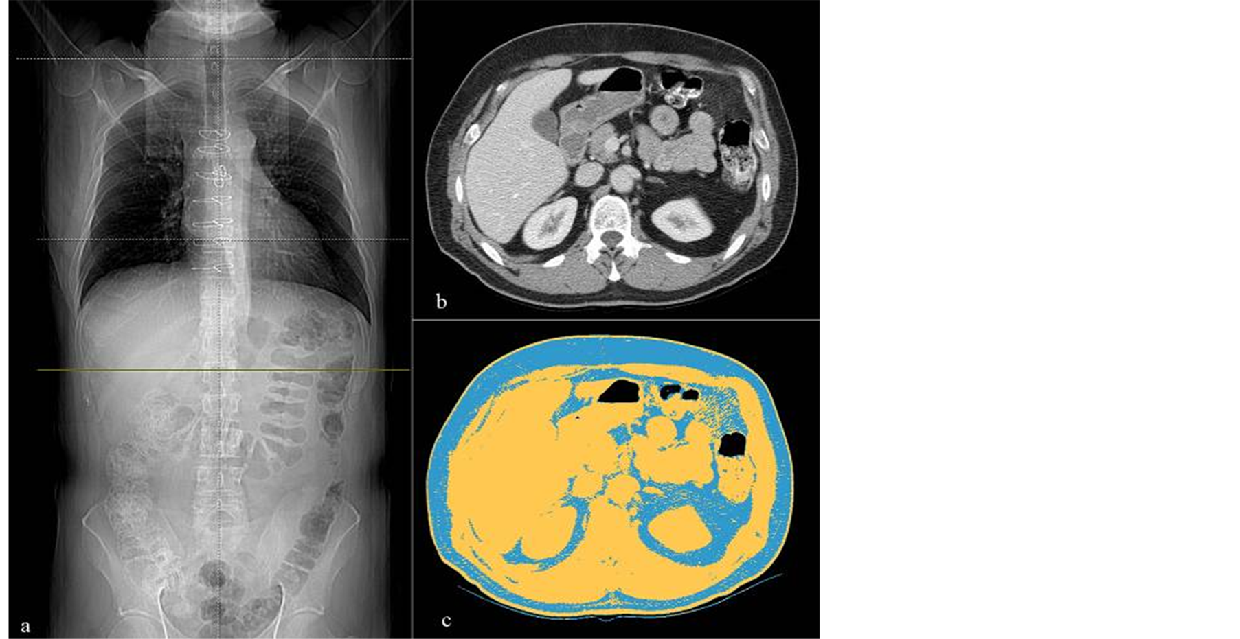
Figure 2. Antero-posterior scout view cross-linked (green line) (a) with the transverse image at the level of the L1 vertebral body (b), and automated segmentation of total body fat of the same transverse image (c).
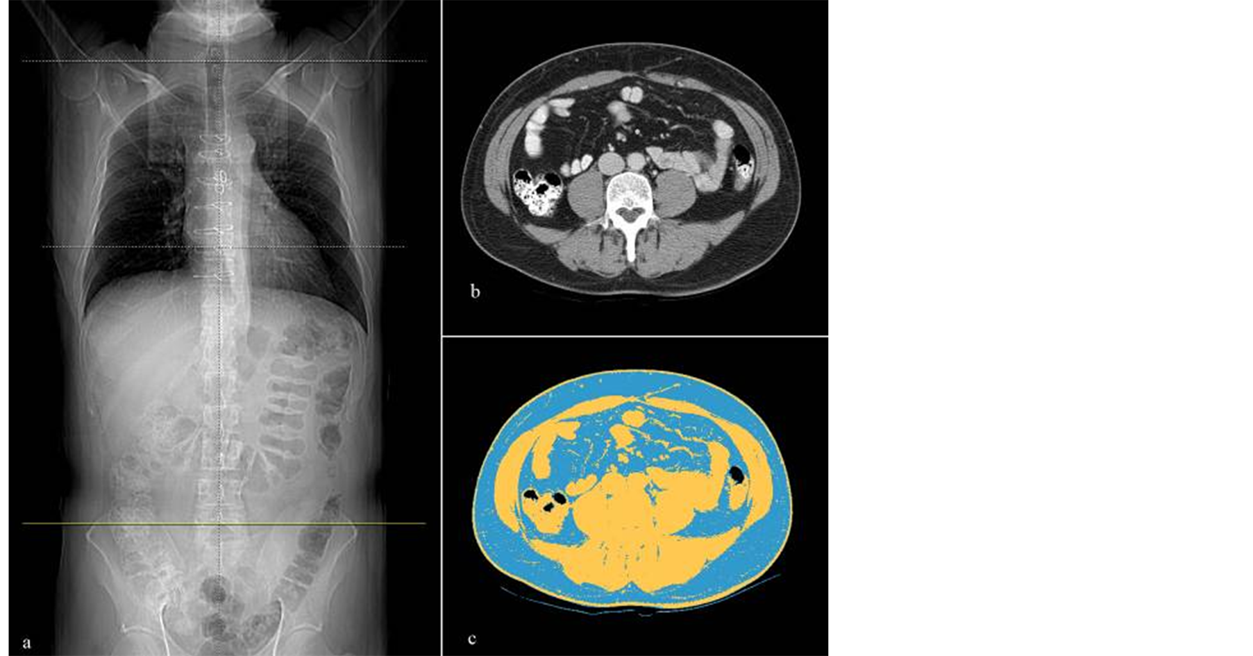
Figure 3. Antero-posterior scout view cross-linked (green line) (a) with the transverse image at the level of the L5 vertebral body (b), and automated segmentation of total body fat of the same transverse image (c).
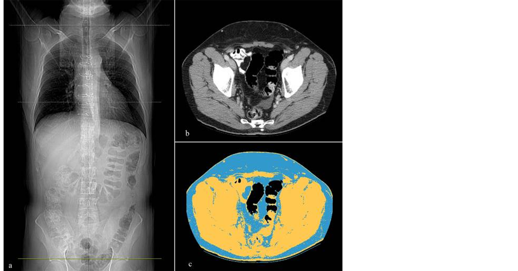
Figure 4. Antero-posterior scout view cross-linked (green line) (a) with the transverse image at the level of the acetabular roof (b), and automated segmentation of total body fat of the same transverse image (c).
three anatomic regions. The higher the ICC value (e.g., >0.8), the lower the variability of the measurements across the five images with each region and thus better agreement between the eLBW measurements. The RC provides the expected absolute difference between any two eLBW measurements for 95% subjects. Thus, the smaller the RC value, the better is the agreement between the eLBW measurements. To determine agreement between mLBW and eLBW, limits of agreement approach by Bland-Altman [18] , for repeated measures were used to determine the expected difference between mLBW and eLBW for 95% subjects in the upper abdomen, mid-abdomen and pelvis regions, separately. To determine the association between patient’s characteristics and

Figure 5. Flow chart of the method used to estimate the LBW from a single CT axial image.
the disagreement between mLBM and eLBM measurements, a binary variable was created to indicate whether the disagreement was greater than the RC of eLBM within the specific region. Logistic regression models were then used to assess the association between age, gender, BMI, total body weight, with the large observed the disagreement between mLBM and eLBM. A generalized estimating equations approach was used in the logistic regression models to adjust for correlations due to multiple eLBW measurements with 5 images within the same patient.
Statistical analysis was performed using a statistical software package (SAS® 9.1, Cary, NC). A two-tailed P-value of less than or equal to 0.05 was considered to indicate statistical significance.
3. Results
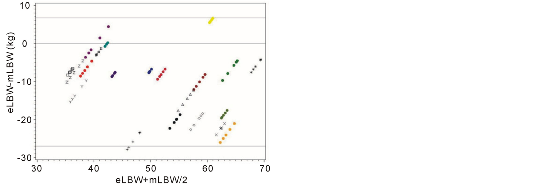
Our study demonstrated no significant different in the eLBWs among five consecutive CT images for each anatomical region. The estimated intraclass correlation coefficients across the five images were 0.87 (95% CI 0.77 - 0.94), 0.97 (95% CI 0.95 - 0.99) and 0.98 (95% CI 0.96 - 0.99) for the upper abdomen, mid-abdomen and pelvis, respectively. The repeatability coefficients across the five images were 10.8, 4.5 and 3.8 kg for the upper abdomen, mid abdomen and pelvis, respectively. This data indicate excellent reproducibility of the method regardless of the section selection in all anatomical regions. The bias (mean differences) and limits of agreement between mLBW and eLBW for the upper abdomen, mid abdomen and pelvis were −9.05 kg (standard deviation [SD], ±8.5 kg) (limits of agreement, −25.6 kg, +7.5 kg) at the level of the L1 lumbar vertebral body, −10.6 kg (SD, ±8.7 kg) (limits of agreement, −27.7 kg, +6.4 kg) at the level of L5 lumbar vertebral body, and +0.5 kg (SD, ±6.8 kg) (limits of agreement, −12.8 kg, +13.8 kg) at the level of acetabular roof (figure 6). Of the three body regions tested, the pelvis yielded the smallest mean difference and the narrowest limit of agreement between mLBW and eLBW. Our data showed a tendency to underestimate patient’s mLBW using the eLBW from the upper and mid abdomen. The results of the linear regression analysis showed a significant positive correlation between eLBW and mLBW at the level of the acetabular roof (correlation coefficients ranging from 0.83 to
 (a)
(a)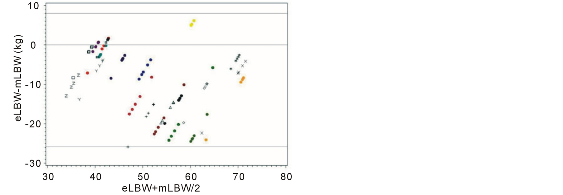 (b)
(b)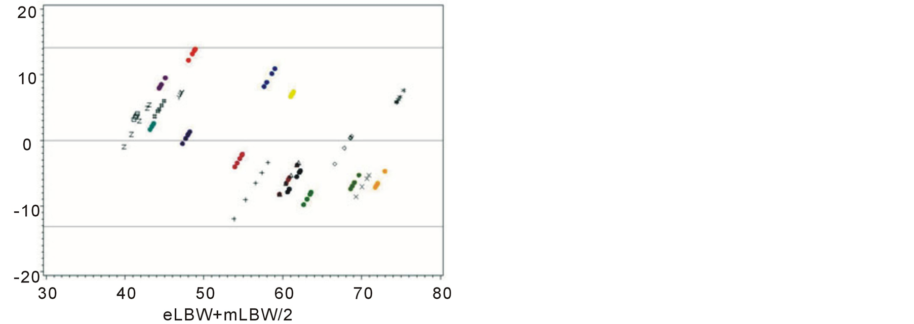 (c)
(c)
Figure 6. Scatter plots (Bland-Altmann plots) of eLBW minus mLBW (vertical axis) against mean of eLBW and mLBW for the upper abdomen (a) mid abdomen (b) and pelvis (c). Symbols with different color represent the CT slices of each patient. The horizontal lines (above and below 0) correspond to the 95% limits of agreement, given by the mean difference plus or minus twice the standard deviation of the differences.
0.87, p < 0.001), with a trend toward underestimating LBW in heavier patients (figure 6(c)). In general, eLBW in the pelvis tended to be lower than mLBW and this finding was more likely in men than in women [male—mean differences, −5 kg (±4.6 kg); female—mean differences, +5 kg (±4.4 kg)]. In order to determine whether the observed large difference is due to patient’s characteristics or not, a binary outcome was created indicating whether the absolute difference between eLBW and mLBW is greater than 4 or not. A unit of 4 is used here because the repeatability coefficient of eLBW in pelvis is 3.8. In the logistic model adjusted for repeated measures and covariates, disagreement between eLBW and mLBW was significantly larger in heavier patients (p = 0.05). However, there was no statistical significant association between age, gender, BMI with large disagreement between eLBW and mLBW.
4. Discussion Our results demonstrate that a precise estimate of patient’s LBW can be obtained from a single transverse CT image, with the highest level of accuracy obtained from images acquired in the pelvis at the level of the acetabular roof. We anticipate eLBW can be used prospectively to determine the contrast material dose and rate during MDCT. The mean difference between mLBW and eLBW (+0.5 kg (SD, ±6.8 kg)) at the level of the pelvis was not relevant, however the reported limit of agreement ((−12.8, +13.8) kg) indicates a possible variability in the estimates and a greater difference between the eLBW and mLBW could occur in some patients. The approach to administer a fixed dose of iodinated contrast medium using a linear scale, based on the assumption of a standard patient size, has been demonstrated to be inappropriate [3] [4] and we believe that our method is a feasible and accurate method for easily estimating LBW in order to tail contrast medium on the basis of LBW, as was recently proposed [2] [3] [5] . In this regard, we think that with a low dose protocol during abdominal and vascular MDCT, estimating LBW at any commercially-available CT workstation should be taken into consideration for daily clinical use because it would not require either any specialized equipment or any time consuming operation. Our study showed decreased agreement between eLBW and mLBW at the level of the upper or mid abdomen, with a tendency to underestimate mLBW from CT images in those regions. We postulate that this finding may be partially related to the inherent limitation of our reference standard, i.e., the FF-BIA measured as the impedance across the lower extremities and pelvis [12] [13] . In contrast to our study, previous studies that have proposed and validated CT as a method to measure body composition indicated the mid-abdomen (i.e., L4-L5 vertebra, umbilicus) as the best body region to predict the total body fat [14] [19] -[21] . These studies [19] -[21] were based on the method described by Borkan et al. in 1982 [14] , which consisted of a manual or semi-automated segmentation technique. An automated quantification of body fat on a volumetric CT has been implemented only recently as a more practical approach [16] . We believe that when the method was proposed the older technique could have been subjected to operator errors and computer-assisted software and thus it was not appropriately developed in order to use them to extract quantitative data precisely. Although CT is still considered one of the most accurate methods for measuring body fat, its clinical utilization for this purpose has been limited, most likely because of CT’s high cost. Though our retrospective analysis has determined clinically promising results, it is presumable that the method, when reproduced with dual-energy MDCT scanners used in conjunction with a low kilo-voltage protocol, could obtain either a greater dose reduction or a better discrimination of the adipose tissue from the other tissues than obtained in our study. Another finding of our study was the trend towards the eLBW underestimating the LBW at the level of the pelvis in overweight and obese patients while TBW showed a significant correlation with eLBW. We don’t know how to explain this result thought we assume that this underestimation of LBW could have resulted from the small number of patients in our cohort. We observe that in men, eLBW in the pelvis underestimated mLBW, possibly as a result of the different body habitus between men (“apple-like” shape) and women (“pear-like” shape) that corresponds to a different body fat distribution [22] . However, this effect is not statistically significant, especially after adjusting for body weight because men tend to be heavier than women. Additionally we found no impact of age on large disagreement between eLBW and mLBW in the pelvis after adjusting for body weight. Since the rate of body fat distribution could vary with age for men versus women [15] , further investigation is warranted on the impact of gender or age on LBW to confirm our results. Some potential limitations of our study merit consideration. First, we could have inaccurately analyzed the CT data of those patients with large body habitus because of possible exclusion of a part of the body from the scan field of view (FOV) and consequently from the thresholding process. It is conceivable that the generally “pear-shaped” body habitus in women, with a distribution of the visceral fat prevalently in the pelvis, could resulted in overestimating the LBW in this location. To minimize the risk of this inaccuracy’s occurring in both men and women, we recommend careful adjustment of FOV in those patients with a large, “pear”-like body habitus in order to include all adipose tissue of the pelvic region in the preliminary image for the thresholding process. Introduction of new MDCT scanners that permit the investigator to chose larger FOVs should minimize this problem. Second, we did not investigate the effect of body fat composition differences associated with some pathological conditions (i.e., Cushing syndrome, metabolic syndrome) [23] [24] in predicting eLBW because of the lack of patients with these diseases in our retrospective population. Finally, the retrospective nature of our study and the small sample size could have increased the influence of several confounding variables (e.g., TBW, BMI and age).
5. Conclusion
In summary, our study demonstrated that a single transverse CT image in the pelvis, specifically at the level of the acetabular roof, can give the radiologist an accurate estimation of LBW. In the future, this technique may be used as an expedited way to estimate LBW as the basis for determining the dose and rate of contrast material for abdominal MDCT.
Acknowledgements
This retrospective study was supported in part by General Electric Healthcare, Inc. The sponsor had no role in the design of the study, development of the model, or interpretation of results. The corresponding author had full control of the data and the information submitted for publication.
References
- Kondo, H., Kanematsu, M., Goshima, S., et al. (2008) Abdominal Multidetector CT in Patients with Varying Body Fat Percentages: Estimation of Optimal Contrast Material Dose. Radiology, 249, 872-877. http://dx.doi.org/10.1148/radiol.2492080033
- Ho, L.M., Nelson, R.C. and Delong, D.M. (2007) Determining Contrast Material Dose and Rate on Basis of Lean Body Weight: Does This Strategyimprove Patient-to-Patient Uniformity of Hepatic Enhancement during Multi-Detector Row CT? Radiology, 243, 431-437. http://dx.doi.org/10.1148/radiol.2432060390
- Yanaga, Y., Awai, K., Nakaura, T., et al. (2009) Effect of Contrast Injection Protocols with Dose Adjusted to the Estimated Lean Patient Body Weight on Aortic Enhancementat CT Angiography. American Journal of Roentgenology, 192, 1071-1078. http://dx.doi.org/10.2214/AJR.08.1407
- Kondo, H., Kanematsu, M., Goshima, S., Tomita, Y., Kim, M.J., Moriyama, N., et al. (2010) Body Size Indexes for Optimizing Iodine Dose for Aortic and Hepatic Enhancement at Multidetector CT: Comparison of Total Body Weight, Lean Body Weight, and Blood Volume. Radiology, 254, 163-169. http://dx.doi.org/10.1148/radiol.09090369
- Kondo, H., Kanematsu, M., Goshima, S., Watanabe, H., Onozuka, M., Moriyama, N. and Bae, K.T. (2011) Aortic and Hepatic Enhancement at Multidetector CT: Evaluation of Optimaliodine Dose Determined by Lean Body Weight. European Journal of Radiology, 80, 273-277. http://dx.doi.org/10.1016/j.ejrad.2010.12.009
- Mattsson, S. and Thomas, B.J. (2006) Development of Methods for Body Composition Studies. Physics in Medicine and Biology, 51, R203-228. http://dx.doi.org/10.1088/0031-9155/51/13/R13
- Burkinshaw, L., Jones, P.R. and Krupowicz, D.W. (1973) Observer Error in Skin Fold Thickness Measurements. Human Biology, 45, 273-279.
- Heyward, V.H. (1996) Evaluation of Body Composition. Current Issues. Sports Medicine, 22, 146-156. http://dx.doi.org/10.2165/00007256-199622030-00002
- Kirkendall, D.T., Grogan, J.W. and Bowers, R.G. (1991) Field Comparison of Body Composition Techniques: Hydrostatic Weighing, Skinfold Thickness, and Bioelectric Impedance. Journal of Orthopaedic & Sports Physical Therapy, 13, 235-239. http://dx.doi.org/10.2519/jospt.1991.13.5.235
- Fields, D.A., Goran, M.I. and McCrory, M.A. (2002) Body-Composition Assessment via Air-Displacement Plethysmography in Adults and Children: A Review. The American Journal of Clinical Nutrition, 75, 453-467.
- Hosking, J., Metcalf, B.S., Jeffery, A.N., Voss, L.D. and Wilkin, T.J. (2006) Validation of Foot-to-Foot Bioelectrical Impedance Analysis with Dual-Energy X-Ray Absorptiometry in the Assessment of Body Composition in Young Children: the EarlyBirdcohort. British Journal of Nutrition, 96, 1163-1168. http://dx.doi.org/10.1017/BJN20061960
- Ritchie, J.D., Miller, C.K. and Smiciklas-Wright, H. (2005) Tanita Foot-to-Foot Bioelectrical Impedance Analysis System Validated in Older Adults. Journal of the American Dietetic Association, 105, 1617-1619. http://dx.doi.org/10.1016/j.jada.2005.07.011
- Lazzer, S., Boirie, Y., Meyer, M. and Vermorel, M. (2003) Evaluation of Two Foot-to-Foot Bioelectrical Impedance Analysers to Assess Body Composition in Overweight and Obese Adolescents. British Journal of Nutrition, 1, 987-992. http://dx.doi.org/10.1079/BJN2003983
- Borkan, G.A., Gerzof, S.G., Robbins, A.H., Hults, D.E., Silbert, C.K. and Silbert, J.E. (1982) Assessment of Abdominal Fat Content by Computed Tomography. The American Journal of Clinical Nutrition, 36, 172-177.
- Grauer, W.O., Moss, A.A., Cann, C.E. and Goldberg, H.I. (1984) Quantification of Body Fat Distribution in the Abdomen Using Computed Tomography. American Journal of Clinical Nutrition, 39, 631-637.
- Zhao, B., Colville, J., Kalaigian, J., et al. (2006) Automated Quantification of Body Fat Distribution on Volumetric Computed Tomography. Journal of Computer Assisted Tomography, 30, 777-783. http://dx.doi.org/10.1097/01.rct.0000228164.08968.e8
- Geraghty, E.M. and Boone, J.M. (2003) Determination of Height, Weight, Body Mass Index, and Body Surface Area with a Single Abdominal CT Image. Radiology, 228, 857-863. http://dx.doi.org/10.1148/radiol.2283020095
- Bland, J.M. and Altman, D.G. (1999) Measuring Agreement in Method Comparison Studies. Statistical Methods in Medical Research, 8, 135-160.
- Tershakovec, A.M., Kuppler, K.M., Zemel, B.S., et al. (2003) Body Composition and Metabolic Factors in Obese Children and Adolescents. International Journal of Obesity, 27, 19-24. http://dx.doi.org/10.1038/sj.ijo.0802185
- Baumgartner, R.N., Heymsfield, S.B., Roche, A.F. and Bernardino, M. (1988) Abdominal Composition Quantified by Computed Tomography. American Journal of Clinical Nutrition, 48, 936-945.
- Seidell, J.C., Oosterlee, A., Thijssen, M.A.O., et al. (1987) Assessment of Intraabdominal and Subcutaneous Abdominal Fat: Relation between Anthropometry and Computed Tomography. The American Journal of Clinical Nutrition, 45, 7-13.
- Power, M.L. and Schulkin, J. (2008) Sex Differences in Fat Storage, Fat Metabolism, and the Health Risks from Obesity: Possible Evolutionary Origins. British Journal of Nutrition, 99, 931-940. http://dx.doi.org/10.1017/S0007114507853347
- Yoshida, S., Inadera, H., Ishikawa, Y., Shinomiya, M., Shirai, K. and Saito, Y. (1991) Endocrine Disorders and Body Fat Distribution. International Journal of Obesity, 15, 37-40.
- Rockall, A.G., Sohaib, S.A., Evans, D., et al. (2003) Computed Tomography Assessment of Fat Distribution in Male and Female Patients with Cushing’s Syndrome. European Journal of Endocrinology, 149, 561-567. http://dx.doi.org/10.1530/eje.0.1490561.