Open Journal of Air Pollution
Vol.2 No.4(2013), Article ID:40470,13 pages DOI:10.4236/ojap.2013.24009
Retrieval of PM10 Concentration from an AOT Passive Remote-Sensing Station between 2003 and 2007 over Northern France
1LOCEANH/IPSL, UPMC/CNRS/IRD/MNHN, Paris, France
2LATMOS/IPSL, UVSQ/UPMC/CNRS, Guyancourt, France
3Institut National de l’Environnement Industriel et des Risques, Verneuil-en-Halatte, France
Email: houda.yahi@locean-ipsl.upmc.fr
Copyright © 2013 Houda Yahi et al. This is an open access article distributed under the Creative Commons Attribution License, which permits unrestricted use, distribution, and reproduction in any medium, provided the original work is properly cited.
Received May 25, 2013; revised June 25, 2013; accepted July 1, 2013
Keywords: Mass Concentration (PM10); Aerosol Optical Thickness (Sun Photometer); Competitive Neural Network; Self-Organizing Map (SOM); Weather Types
ABSTRACT
A method of retrieving PM10 particles concentrations at the ground level from AOT (Aerosol Optical Thickness) measurements is presented. It uses data obtained among five years during 2003 to 2007 summers in the Lille region (northern France). As PM10 concentration strongly depends on meteorological variables, we clustered the meteorological situations provided by the MM5 meteorological model forced at the lateral boundaries by the operational NCEP model in eight classes (local weather types) for which a robust statistical relationship between AOT and PM10 was found. The meteorological situations were defined by the hourly vertical profiles of temperature and (zonal and meridian) wind components. The clustering of the weather types were obtained by a self-organizing map (SOM) followed by a hierarchical ascending classification (HAC). We were then able to retrieve the PM10 at the surface from the AERONET AOT measurements for each weather type by doing non linear regressions with dedicated SOMs. The method is general and could be extended to other regions. We analyzed the strong pollution event that occurred during August 2003 heat wave. Comparison of the results from our method with the output of the CHIMERE chemical-transport model showed the interest to tentatively combine these two pieces of information to improve particle pollution alert.
1. Introduction
Air pollution in cities has a major impact on human health and constitutes one of the major environmental and public-health issues human society has to address today. The abundance of fine particles is one of the indicators of degradation of air quality and is therefore subject to an official standard: PM10 and PM2.5 are the masses (in micrograms) per unit volume (cubic metres) of particulate matter (PM) of diameter less than 10 µm and 2.5 µm, respectively. PM10 measurements are easily made in airquality networks using TEOM (tapering element oscillation microbalance). PM10, especially, encompasses a wide range of particle types in terms of size (coarse, fine, and ultrafine) and can differ from chemical composition (dust, combustion particles, marine primary particles, secondary organic aerosol, secondary inorganic aerosol) and sources (natural or anthropogenic) as car traffic, industrydomestic household). This complex composition hampers the understanding of PM10 as a function of local sources, long-range transport and meteorology for a given site. In practice, values exceeding the legal limit, particularly the daily limit of 50 µg/m3, have frequently been measured at air-quality monitoring stations in many European Community member states. Air-quality monitoring stations have been established in major cities and provide information required for issuing a pollution alert. But measuring stations are sparsely distributed and do not provide sufficient data for mapping particle concentration, since air quality can be highly variable both in space and in time. However, Earth observation by satellite sensors could be a valuable tool for assessing and mapping air pollution. The key parameter for this purpose is the horizontal distribution of columnar aerosol optical thickness [1], but the relationship between the aerosol concentration measurement (PM10) and aerosol optical thickness (AOT) is complex since AOT is an integrated measurement from which PM10 is a priori but one contribution. For that purpose, to investigate the statistical relationship between PM10 and AOT, we used the atmospheric optical thicknesses as estimated from ground based passive remote-sensing instruments: sun photometer measurements. Studies devoted to the relationship between PM10 concentration and atmospheric optical thickness measured by passive remote-sensing instruments have received considerable attention and have underlined a high potential for using aerosol optical properties in air-quality studies ([2-5] found that a simple linear regression between PM10 and aerosol optical thickness (AOT) failed to satisfactorily describe the relationship between these quantities). They showed a non linearity in relationship between PM10 and AOT and a real improvement by taking into account auxiliary parameters such as the meteorological variables (e.g. temperature, wind vector, atmospheric moisture content, aerosol sources…) because the atmospheric pollutants concentration vary in space and time, due to the atmospheric forcing conditions.
Moreover, vertical profiles of PM10 concentration in the boundary layer need to be taken into account since they characterize height variability of the pollutants concentration [6,7]. Such profiles are closely related to the atmospheric stability and consequently to the intensity of vertical mixing.
Synoptic climatology approaches have become popular for evaluating impacts of large-scale meteorological conditions on local environmental phenomena, such as air pollution, since they influence the regional and local atmospheric conditions which are characterized by different micrometeorological behaviours. This led the airquality scientific community to recognize atmospheric circulation (at meso and large scale) as an important driver of local air pollution. As an example, [8] studied the relationship between large-scale circulation and air pollution in Melbourne, Australia. [4] showed that, in the small domain of Lille area, in northern France, a statistical relationship between PM10 and AOT could be established by decomposing the meteorological situations into weather types. In the present study, we develop and apply for the summer periods (five years observation) from 2003 to 2007 the method already initiated by [4]. We also analyze the interest to combine our method with pollution forecast models as CHIMERE, particularly in case of a strong pollution event occurrence probability.
In Section 2, to better present and to explain the utilized method, we have preferred to first show the data used and then the method since the latter is very dependent on the used data. Three summer data sets have been used and applied to our methodology. We present successively the surface measurements of PM10 which are the basic surface measurements and then AOT observations used in this study. Then the different model inputs are described.
In Section 3, the methodology is described and applied to the dataset.
Section 4 presents results of PM10 retrieval from AOT and hence the relevance and the precision of the method Section 5 is a discussion of PM10 measurements and PM10 chemical model estimates. Particularly as we were only users of CHIMERE output, we analyze the difference between PM10 observations and model output. For that purpose 2003 pollution event is considered in relation with CHIMERE forecast modelling results.
We also consider the interest to combine our retrieval method with chemical model forecast in case of high particles pollution level probability.
We then carry out some conclusions.
2. Data Used
2.1. Ground Level Measurement of PM10 Particulate Concentration
The reference pollution network measurements were performed at 2 m above the ground surface using a Tapering Element Microbalance system (TEOM), see [9]. We took into account all the available data in the Lille region: five PM10 stations. All the PM10 data are averaged during one hour. 11,040 hours corresponding to 92 days during each 2003-2007 summers are here considered.
Stations are located in a 15 km × 15 km area (see Figure 1) and are considered to represent particles pollution representative of Lille area using a spatial average [4] which will be quoted PM10-Obs in the paper. It has to be remarked that PM10 surface measurements are always available whatever the meteorological situation is.
2.2. Sun Photometer AOT Observations
AOT are estimated using the AERONET regional net-
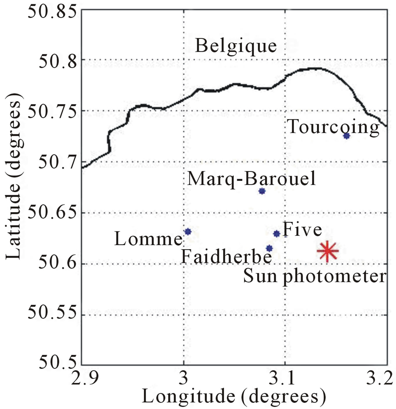
Figure 1. Area of study and location of the five measurement stations and the sun photometer at Lille region.
work which provides globally distributed near-real-time observations of aerosol spectral optical thickness by measuring the direct solar radiation extinction with a relative accuracy of 1% ([10]). We used hourly measurements (automatically made between 05:00 and 18:00) at three different wavelengths (430 nm, 760 nm, 870 nm) by a single sun photometer (referred as the AERONET data) mounted on the roof of a three-storey building in the Lille region. A full description of the instrument and of the retrieval procedure can be found in [10]. Owing to cloud cover, we only collected 836 hourly measurements at the three wavelengths during the observation period. AOT observations of this Lille AERONET station will be used in relation with PM10-Obs.
2.3. Large-Scale Data: Output of the Atmospheric and Chemical Transport Models and Auxiliary Meteorological Parameters
In our study we used the vertical profiles of meteorological variables simulated by MM5 (http://www.mmm.ucar.edu/mm5/) and the surface values of PM10 simulated by the chemical transport model CHIMERE.
The hourly gridded meteorological data analysis (vertical profiles of temperature, zonal and meridional wind components) from the regional atmospheric model MM5 (2003 to 2007) forced at the lateral boundaries by the operational NCEP (National Center for Environmental Prediction)/NCAR (The National Center for Atmospheric Research) model, were used to determine the weather types affecting the Lille area.
The atmospheric aerosol concentration was simulated by the chemistry-transport model CHIMERE. This model was forced with data and observations provided from different sources:
1) Biogenic and anthropogenic emission data by the data base EMEP (European Monitoring and Evaluation Programme).
2) Meteorological observations by the European Range Weather (ECMWF) analysis.
3) Land topography by a terrain data base (MNT).
The output of the atmospheric model (MM5) and that of the chemical transport model CHIMERE were obtained by the runs made in the framework of the GEOMON program (http://www.geomon.eu/) over a domain covering a large part of Europe (35˚N - 70˚N, 10˚W - 35˚E). The MM5 model used twenty vertical sigma-pressure levels with equivalent Z height levels (in metres): from 46 m up to 11,725 m with a variable vertical resolution from typically 50 m to 100 m in the lower part of the atmosphere up 1800 m at the atmosphere top. Outputs are hourly, with a spatial resolution of 0.5˚ × 0.5˚ (about 55 km × 55 km). In the Lille region, for the five summers of the years 2003-2007 (June to August), we obtained 11,040 model outputs collocated with the 11040 PM10- Obs. Detailed description of the model configuration and performances over Europe has been presented in previous studies [11,12]. A first validation of the ability of CHIMERE to simulate aerosol concentration was carried out by [12] who compared the CHIMERE PM10 values against the PM10 values measured by the EMEP station network in 1999. They found correlation coefficients ranging between 0.30 and 0.70. The mass of aerosol was underestimated mainly in southern Europe where the concentration of Saharan dust can be important. However, relative errors in daily PM10 concentration were from 30% up to 80%, but EMEP stations are outside France. More recent results from CHIMERE on PM10 forecast have shown improved PM10 estimations, [13].
We then strictly apply our method to the data described.
3. Analysis Methods
PM10 concentration retrieval from AOT measurements is a difficult task, since the physical relationship between AOT and PM10 both depends on intrinsic PM10 properties which are surface measurements, on particles which are integrated inside the photometer beam, and on meteorological variables. [4] showed that a quite simple relationship between sun photometer observations and groundlevel PM10-Obs concentration can however be used with a minimum of meteorological weather types.
As in [4] we clustered here the 11040 meteorological situations provided by the MM5 meteorological model output for the summers of 2003-2007 by using a selforganizing map (SOM). Since the size of the data set we have is much larger than the one used by [4], we adopted a more systematic approach. We determined a huge number of prototypical meteorological situations using SOM and then reduced this number using a hierarchical ascendant classification (HAC).
SOM is an unsupervised classification method composed of a competitive neural network structured in two layers, [14]. The first layer represents the input layer, which receives the data (here the meteorological situations; Figure 2) and the second one is a neuron grid, usually 2-dimensional, with a topological ordering of the typical meteorological situations. It summarizes the information contained in the multivariate learning set 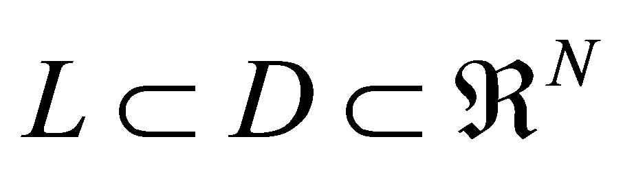 (L being the 11,040 meteorological situations) by producing a small number, m, of reference vectors, Wj (0 < j ≤ m), that belong to D and are statistic cally representative of the learning set. Each neuron represents a subset (or a class) of L that assembles data having common statistical characteristics, which are synthesized by its reference vector, Wj. The topological order means that similar situations of L are mapped onto
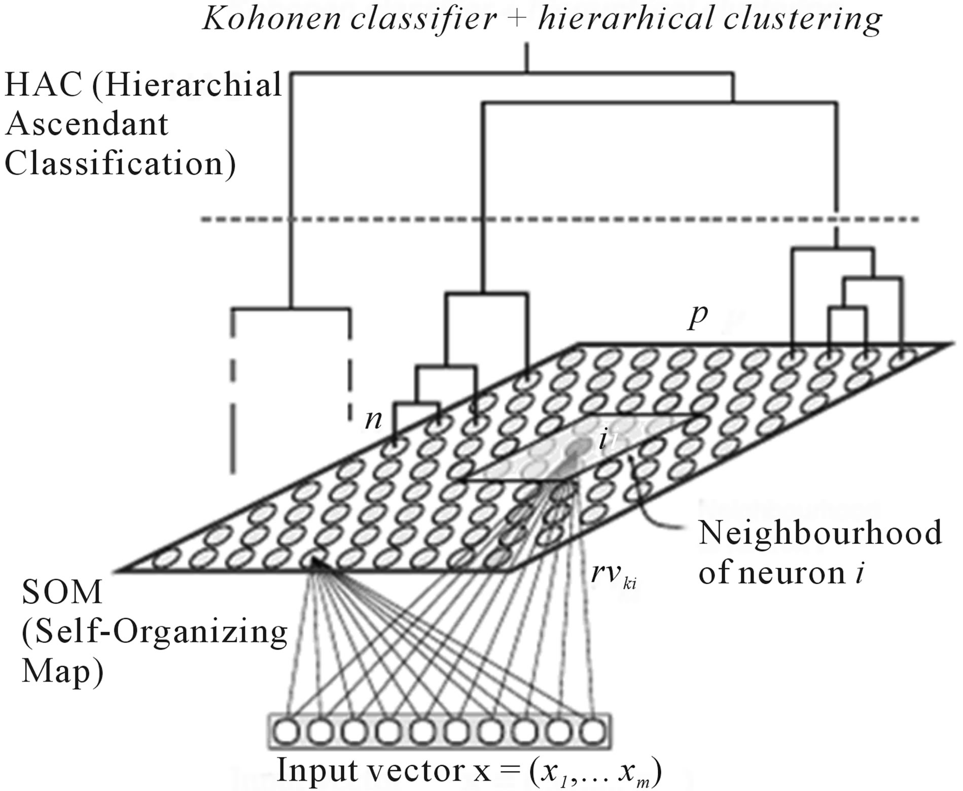
Figure 2. Structure of the SOM map. The network comprises two layers: an input layer used to present observations and an adaptation layer for which a neighborhood system is defined (distance, d, between neurons and a neighborhood function). The number of neurons in the input layer is equal to the dimension of a meteorological situation (n = 720, corresponding to the 60 component vectors defined on the 12 grid points of the geographical map). Each neuron, i, of the map is fully connected to the input layer. It is associated with a group that is represented by a reference vector, rv, which is represented by the weights of the connexion to the input layer. The neurons are clustered in classes by a hierarchical ascendant classification.
neighbouring regions on the SOM map, while dissimilar patterns are mapped farther apart. The number of neurons determines the granularity of the mapping, which in turn is responsible for the accuracy and the generalization capabilities of the SOM map. The reference vectors, Wj (0 < j ≤ m), are determined from L, through a learning process [14] by minimizing a non-linear cost function. For a given training pattern,  , presented to the network, the Euclidian distance for all the reference vectors is computed and the closest reference vector, Wj, is selected. This reference vector is called the best matching unit (BMU) and its associated neuron is denoted the winning neuron. After finding one BMU, all the reference vectors, Wj, of the SOM are updated: the BMU and its topological neighbours are moved in order to better match the input vector. At the end of the training process, the SOM map provides topological (neighborhood) relationships among all the different neurons (or classes). A classification can be thus applied to analyze new meteorological situations. Analysis of a new situation is done by introducing it into the input layer and computing its BMU. The large number of subsets provided by the SOM map allowed us to take into account the complexity of the dataset, but may have prevented us from synthesizing some meteorological information embedded in the learning set. To counteract this difficulty, we decided to aggregate this large number of subsets into a smaller number of types based on the similarities of the subsets. We thus extracted a few pertinent “Weather Types” from the subsets by clustering subsets having similar statistical properties, with the expectation that the “Weather Types” could be associated with common meteorological characteristics. To simplify, we find a “weather type” from a statistical point of view which has to correspond to a relevant meteorological type or situation.
For that, we used a hierarchical ascendant classification (HAC; [15]) using the Ward, 1963 distance for the intra-class similarity. We aggregated the 10 × 10 neurons into eight significant types. The number of types was decided by choosing the most significant discriminative partition with respect to the dendrogram of the HAC.
In our study, we applied the SOM algorithm to the vectors representative of meteorological situations (vertical profiles of temperature, of zonal and meridional wind components). For that purpose, we used the atmospheric output provided by the numerical atmospheric model MM5 by taking into account 12 grid points of that model around the Lille area (see Figure 3): the blue grid cell corresponds to the area in the vicinity of Lille where the five PM10 measuring stations and the sun photometer are situated. These twelve cells allow us to take into account the local weather conditions (the four green cells contiguous to Lille) as well as the meso-scale weather situations. Each input vector of SOM1 is thus constituted by three vertical profiles of atmospheric parameters (temperature, meridional and zonal wind components at twenty vertical levels) at each of the 12 grid cells (Figure 3). The 720 (20 × 3 × 12) components of the input vector of SOM are outputs of MM5. At the end of the learning phase, the 10 × 10 SOM map (denoted SOM1) provides 100 typical meteorological situations representative of the 2003-2007 summer periods. These typical meteorological situations were reduced into eight groups by using a hierarchical ascendant classification. A summary of the

Figure 3. Representation of the Lille area and the coloured grid cells for which we considered the meteorological profiles for clustering the meteorological situations into weather types. The blue grid cell corresponds to the Lille area.
methodology we used is given in Figure 4.
We then retrieved the PM10-Obs from the corresponding AOT measurement by applying a dedicated SOM for each weather type.
In the next section we describe more precisely the different data which were used to apply our method for the five summers analyzed.
4. Results and Discussion
4.1. Classification into Weather Types
In Figure 5 we have represented the mean wind and temperature maps for three weather types, for the five summer periods under study. Notice that 1) corresponding to weather type 2 corresponds to temperature in the Lille region close to 14˚C while wind speed is close to 2 m/s and wind direction southward. We remark that the iso-wind lines have rather a zonal behaviour. For 2) corresponding to weather class 4 the temperature is close to 18˚C while wind speed is close to 2 m/s with rather a meridian structure (wind blowing eastward). For 3), the weather class 7, the temperature is around 20˚C while wind speed is very low close or smaller than 1 m/s and the wind speed is homogeneous in the North of France. We observe that these classes are well differenced from temperature and wind and must correspond to different transport and diffusion characteristics corresponding also to particular micrometeorological characteristics and/ or chemical mechanisms.
We obtained 836 collocated AOT and PM10 measurements associated with their corresponding meteorological situations. Each situation is associated with a weather type. We were thus able to characterize each weather type by a pollution level. Table 1 shows the meteorological characteristics and the mean AOT and PM10 values associated with each weather type. The computed weather types seem to correspond to well-characterized AOT and PM10 values. In the following, we suggest to take these mean AOT values as pollution indices:
Index 1: AOT < 0.11, corresponds to a low pollution level (weather type 1).
Index 2: 0.11 ≤ AOT < 0.17 corresponds to a moderate pollution level (weather types 2 and 3).
Indice 3: 0.17 ≤ AOT < 0.23, corresponds to a high pollution level (weather types 4 - 6).
Indice 4: AOT > 0.23 corresponds to a very high pollution level (weather types 7 and 8).
The clustering into weather types allows us not only to associate a pollution index with each weather type, but to also characterize it by a typical optical thickness spectrum at three wavelengths (430 nm, 760 nm, 870 nm), as shown in Figure 6.
The eight spectra presented in Figure 6 are well identified. They are characteristics of each weather type. For the long observed situations which correspond to five summer periods we have found that relationships between the PM10 and the AOT measurements exist for each weather type.
4.2. Retrieval of PM10-Obs from AOT Measurements
The relationship between PM10 concentration and AOT measurements depends on meteorological parameters.

Figure 4. Schematic representation of the method; the top part of the figure represents the classification process.
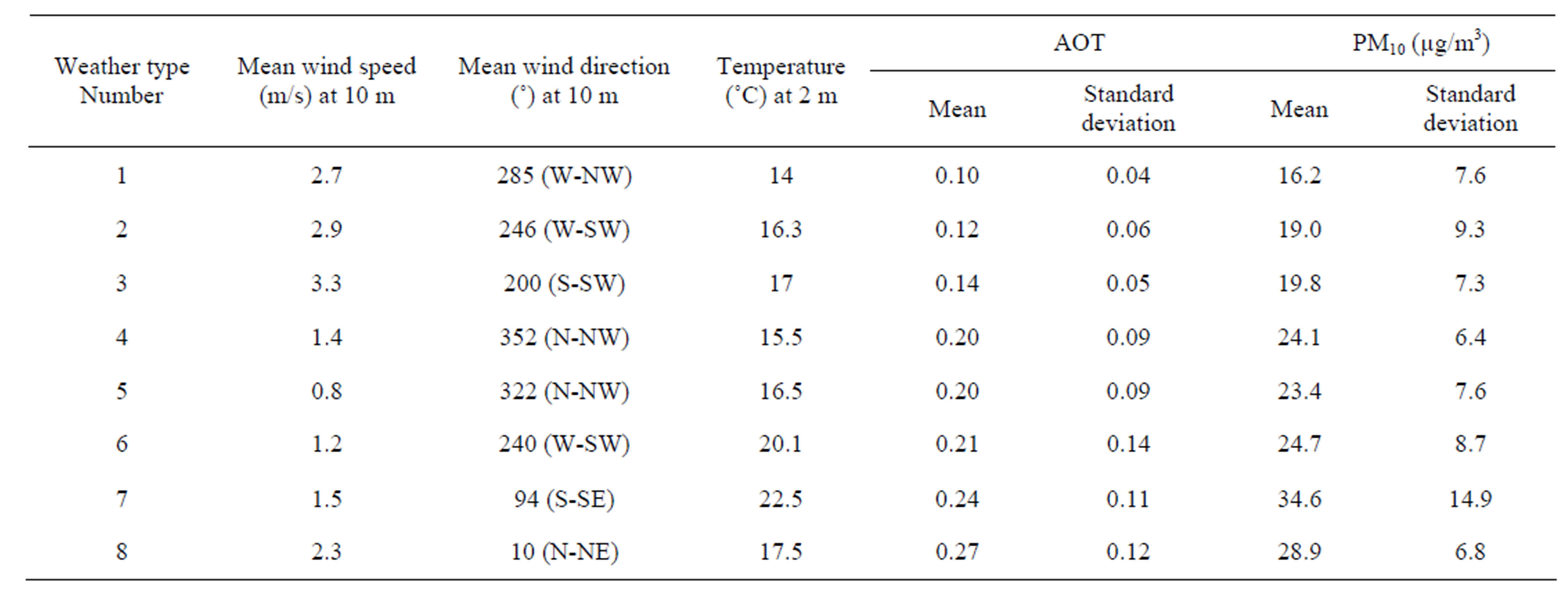
Table 1. Characteristics of the eight weather types.
 (a)
(a)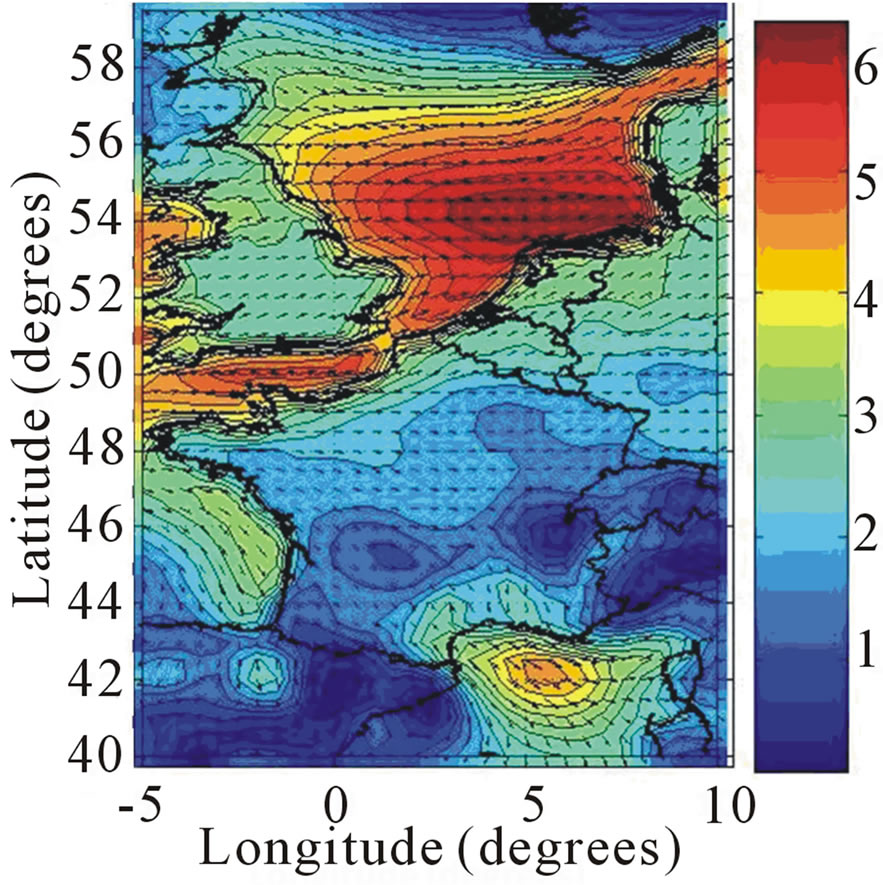 (b)
(b)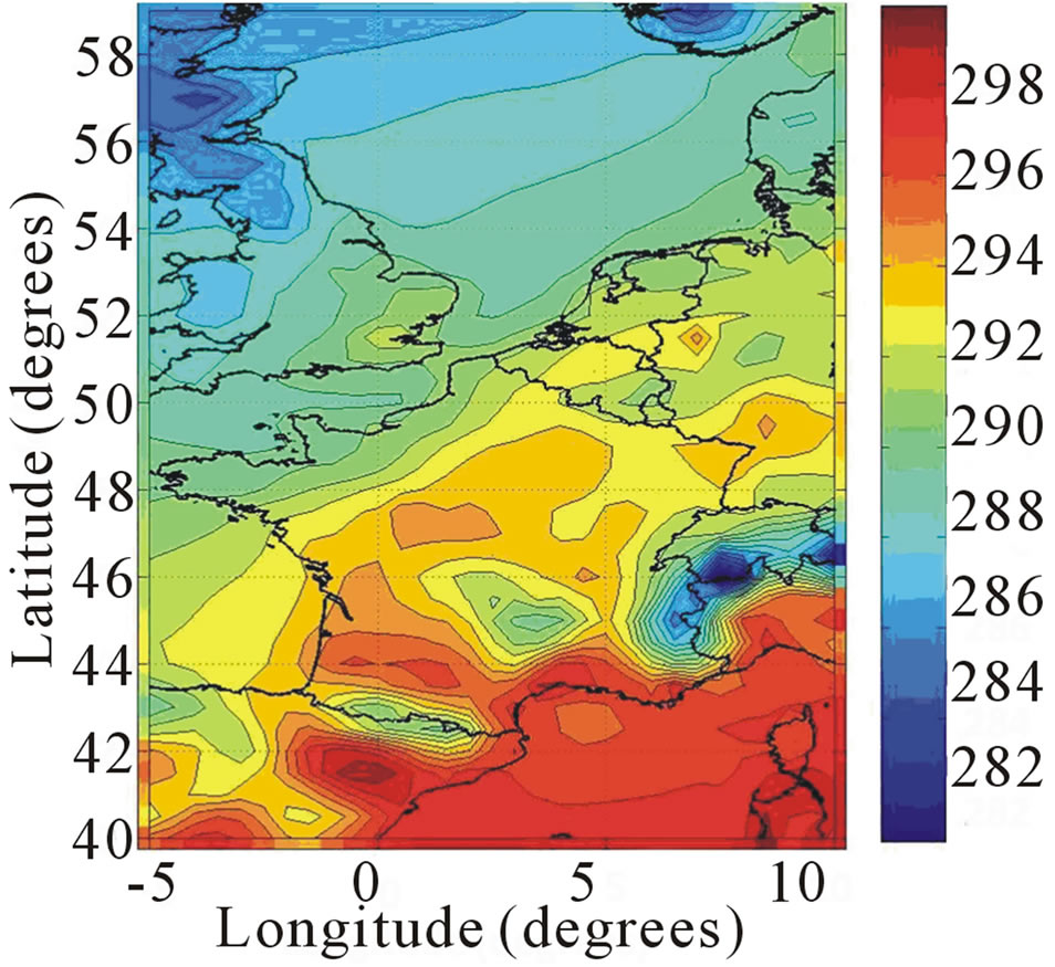 (c)
(c)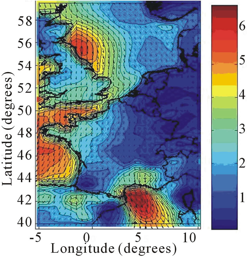 (d)
(d)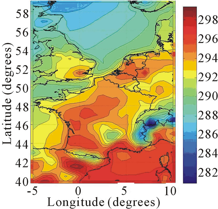 (e)
(e)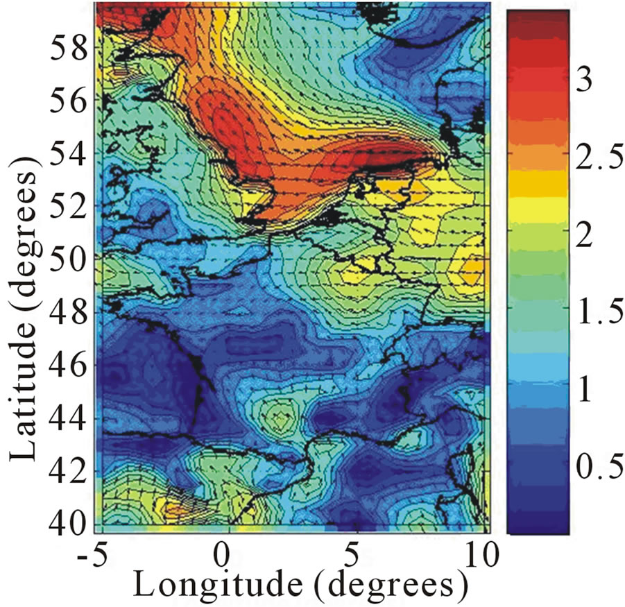 (f)
(f)
Figure 5. Mean winds and temperature maps obtained over France for three weather types: (a), (b) “weather type 2”; (c), (d) “weather type 4”; and (e), (f) “weather type 7”. The colours indicate the wind and temperature intensity.
This relationship must be simplified for each weather type, which has similar meteorological structures. The retrieval of the PM10 concentration from the AOT measurements was done by determining eight different relationships, one for each weather type. For each weather type, N (N = 1, 8), the inversion was done by associating AOT and the local meteorology with the corresponding PM10-Obs using eight dedicated SOM maps (denoted SOMW-N in the following). If the decomposition in weather type has removed the effect of meteorological parameters at first order, second order effects may remain and must be introduced in the retrieval process in each class.
The inputs of the eight SOMW-N were the AOT measurements at three different wavelengths, the meteorological parameters (zonal and meridional components of the wind at three different vertical levels, and the ground-level temperature) at Lille. Since each data is associated with a PM10-Obs concentration, each neuron of SOMW-
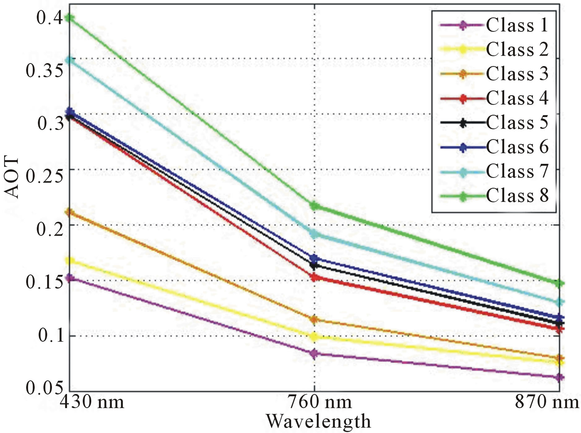
Figure 6. AOT spectrum at three wavelengths (430 nm, 760 nm, 870 nm) for the eight weather types (C1 - C8).
N has captured PM10-Obs information and can be characterized by the mean of these captured PM10-Obs which are outputs of SOMW-N. In order to obtain a good accuracy in the PM10 retrieval, we used 6 × 6 neurons SOMW-N maps.
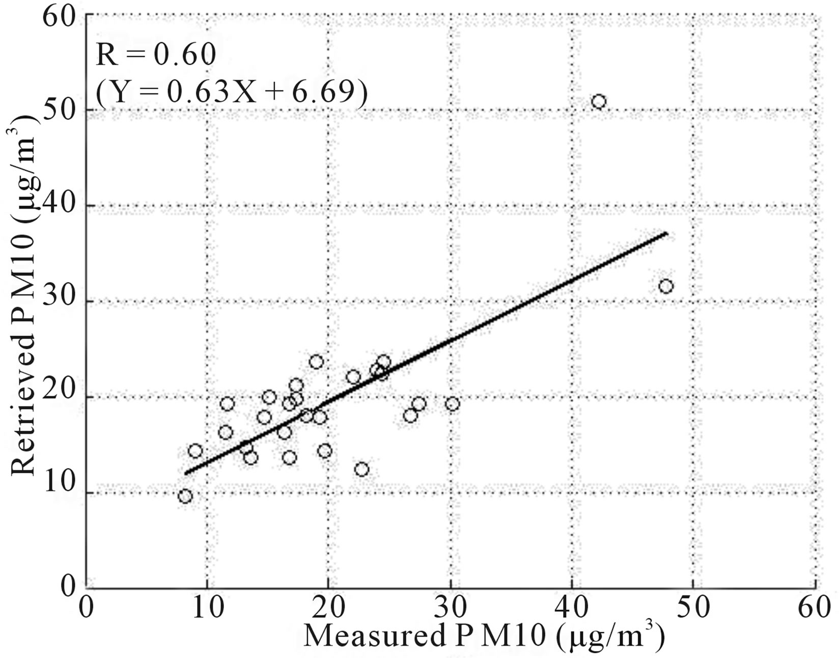
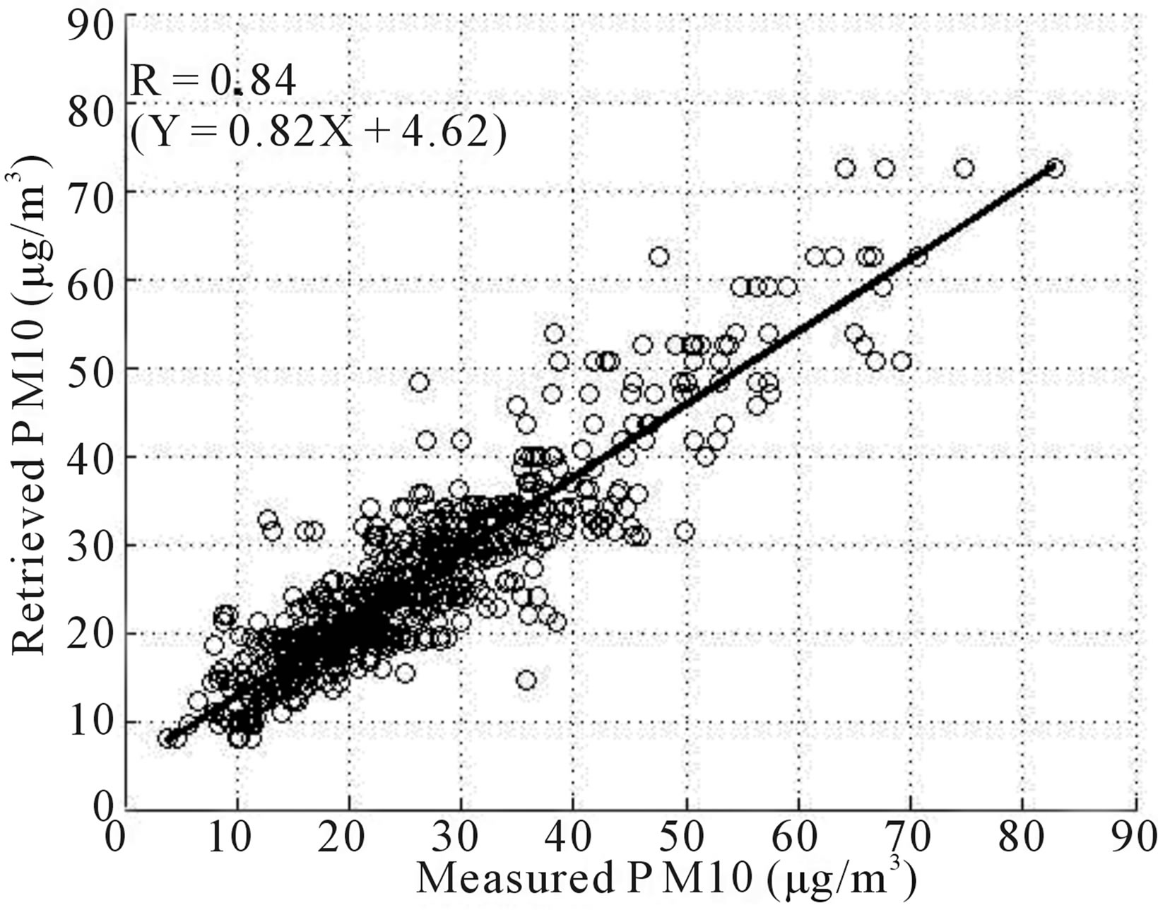
For each SOMW-N, Table 2 shows the number of collocated data pairs (PM10-Obs and AOT) used for the learning and the test phases for each weather type. The performances of the inversion computed on the test datasets are satisfactory for most of the classes. In Figure 7, we show the scatter plot for the mass concentration PM10 retrieved with respect to PM10-Obs, for weather types n°2, n°4 and n°7, corresponding to the three weather types presented in Figure 5. In order to check the overall performance of the methodology, we show the scatter plots for the learning (Figure 8(a)" target="_self">Figure 8(a)) and test set (Figure 8(b)) obtained by pooling the eight inversions we processed. Table 3" target="_self"> Table 3 shows some statistical estimators (see Annex 1 for the definition of the statistical estimators) computed on the learning and the test sets, allowing us to estimate the accuracy of the AOT – PM10 relationship. The relative root mean square error RRMSE (25%, for the test set) and the correlation coefficient (0.80, for the test set) show that the performances are satisfactory. Performances of the learning and the test sets are of the same order, indicating that the non-linear regression is quite stable. These performances could be improved by increasing the size of the learning set.
We have shown that PM10 obtained with our method are relevant and accurate. Therefore we examine now how our method can be used for particles pollution alert.
5. Uses of the Method in Case of Pollution Alert
5.1. PM10 Estimate Use for Forecast
To be able to monitor a pollution threshold over which
 (a)
(a)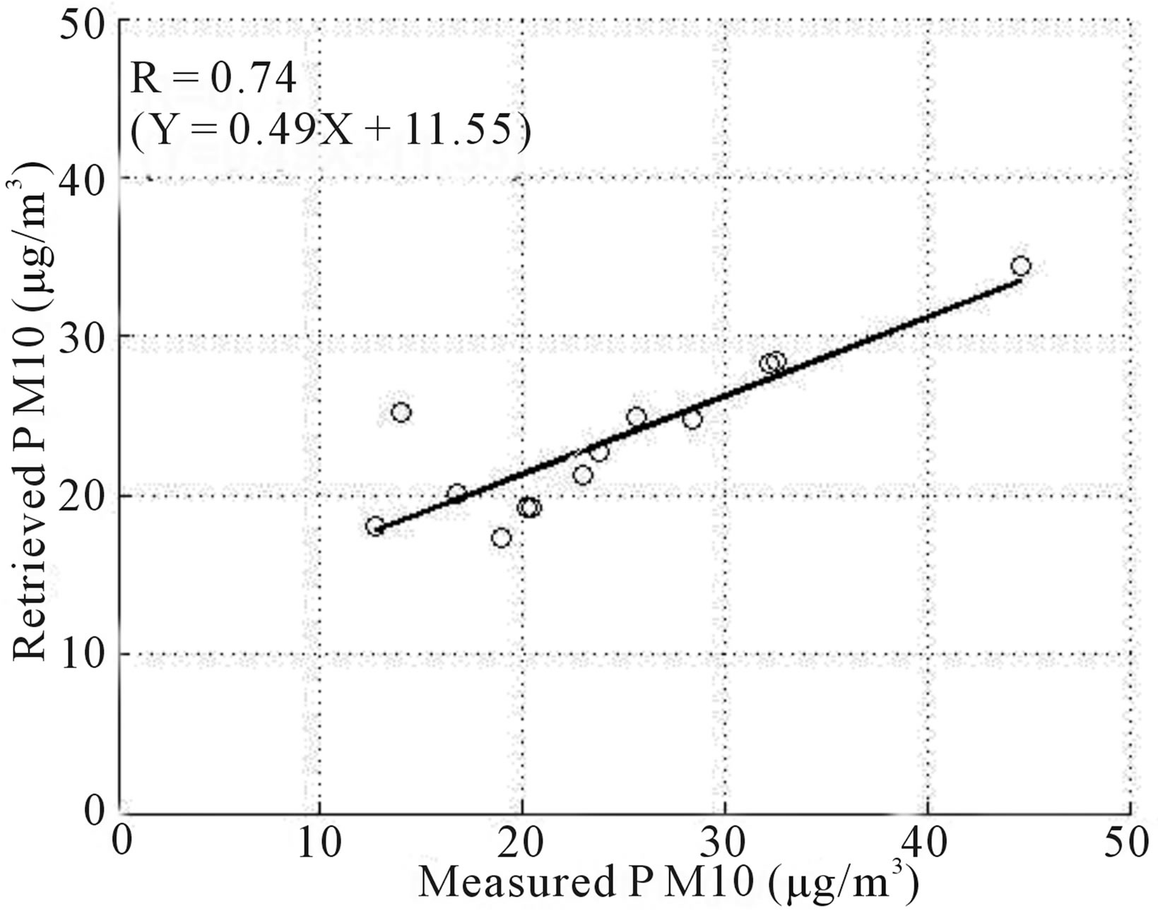 (b)
(b)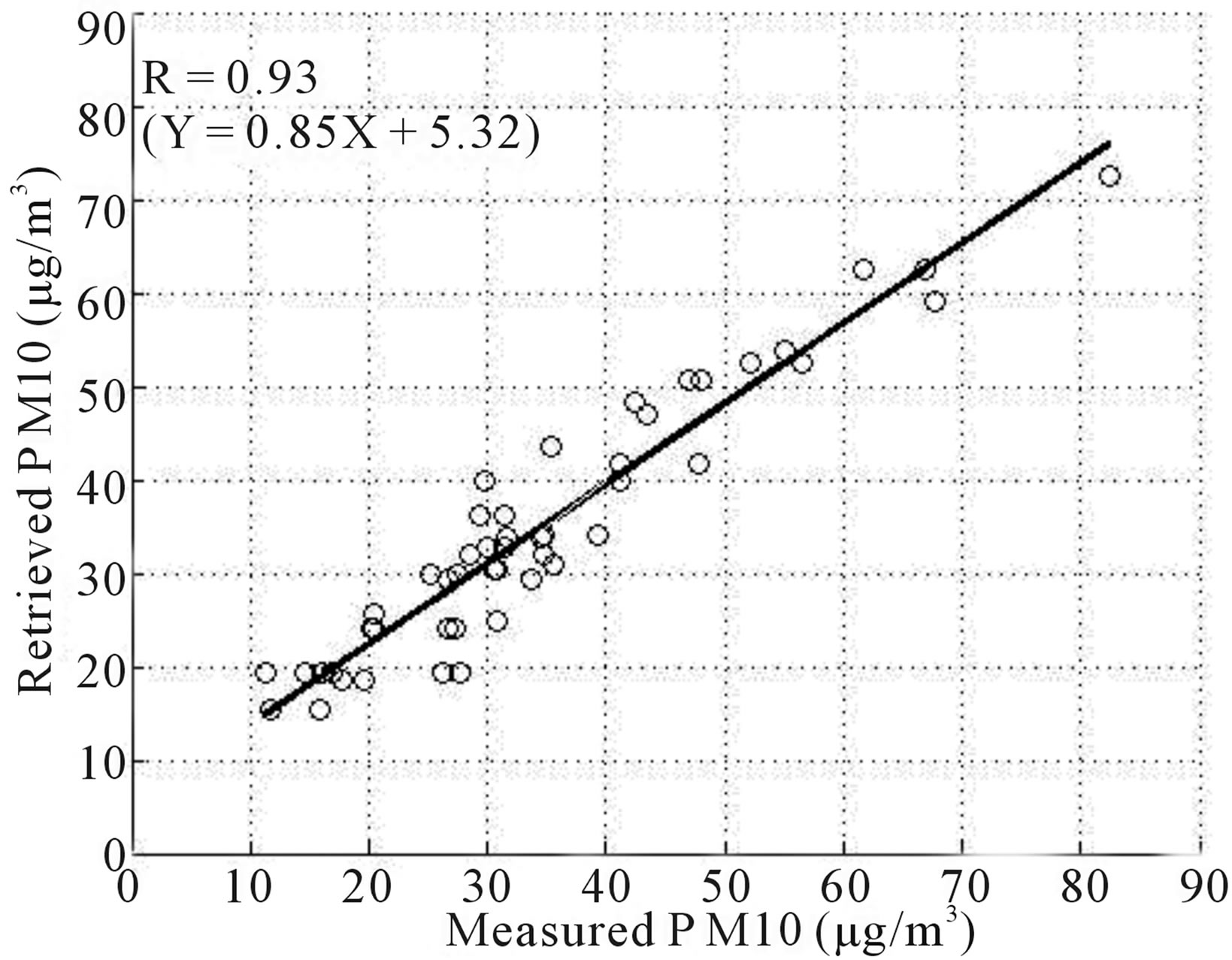 (c)
(c)
Figure 7. Retrieved PM10 versus measured PM10 obtained with SOMW-N trained on the Lille data set (AOT (AERONET data) + Meteorological variables) for the weather type 2, b the weather type 4, and c the weather type 7.
 (a)
(a)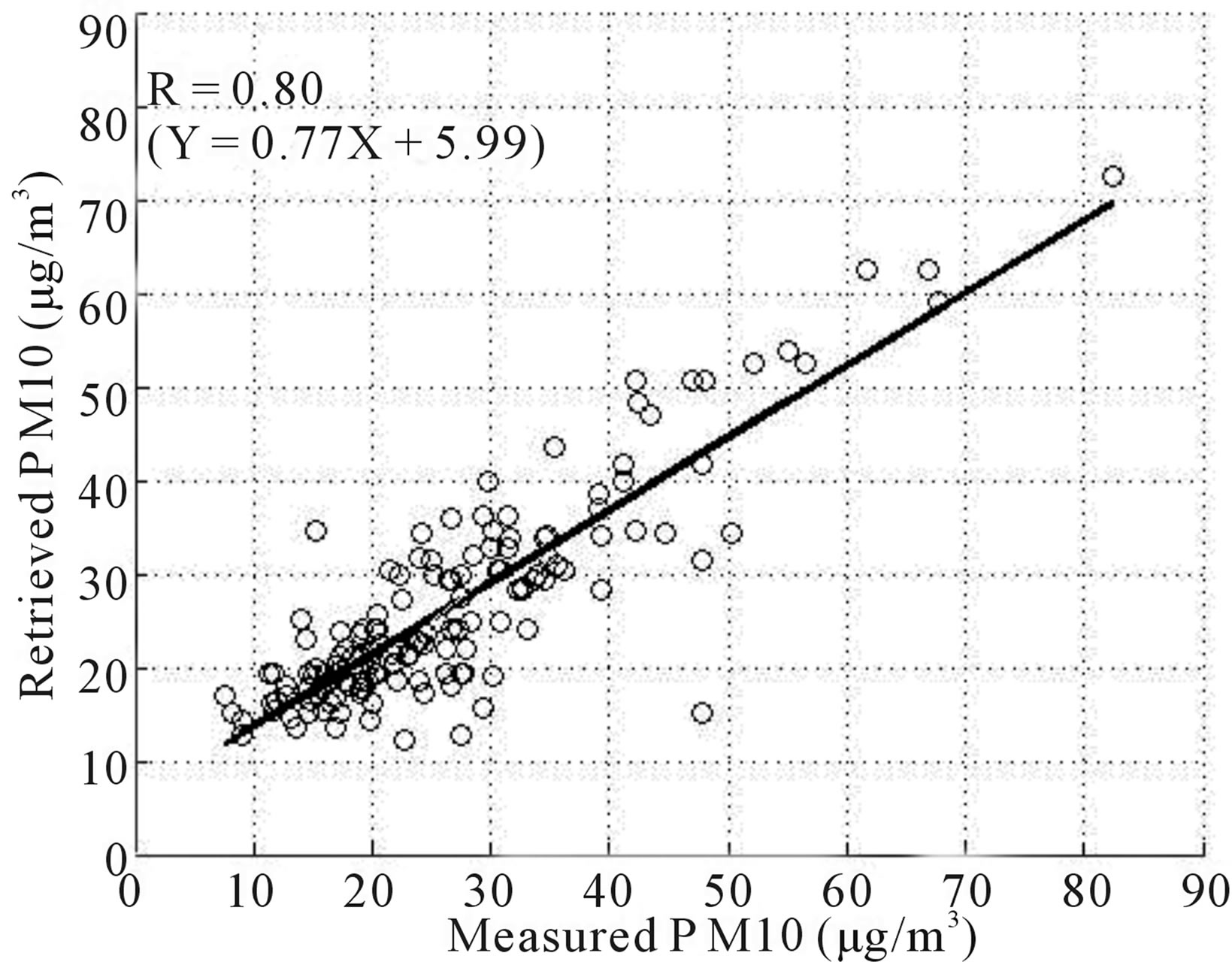 (b)
(b)
Figure 8. Scatter plot of the PM10 retrieval (measured PM10 versus retrieved PM10 from AOT) for the learning set (a) and the test set (b) merging the eight inversions processed.

Table 2. Number of collocated data for each weather type.
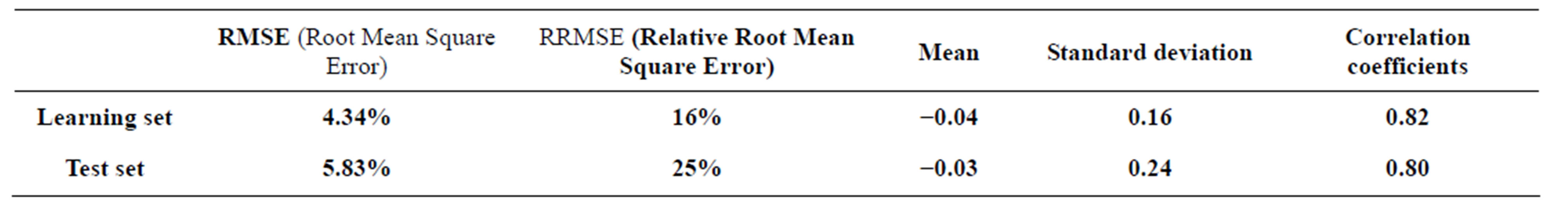
Table 3. Performances of the AOT models for the learning and test sets.
some damage to human health might occur following the World Health Organization (OMS) standards, we have to examine the PM10 retrieval characteristics. First, since the classification of the meteorological situations in weather types allows us to establish a pollution index (1 to 4) from the meteorological variables only, we can envisage forecasting a pollution index for the next day by projecting the forecast meteorological variables for the following day onto SOM1. The weather type associated with the projected meteorological situation is linked to a pollution index, which will be the “pollution forecast index”. Second, we can use the AERONET observations, which are easy to invert with the method we have developed. The PM10 concentration can be estimated with a good accuracy from the AOT observations.
To evaluate the operational use of our method for forecasting the PM10 concentration, it is then necessary to analyze the CHIMERE PM10 forecast in the Lille region and to present comparisons with PM10 measurements and estimates.
5.2. CHIMERE Model PM10 Output
In order to build an air-quality modelling system with confidence for forecasting pollution events, we evaluated the CHIMERE model performance against direct measurements. For that purpose we used the 836 PM10-Obs (mean hourly concentrations measured at the five urban ground stations in the Lille region) collocated with the AERONET observations. This data set was also collocated with the CHIMERE output. Figure 9 presents the histogram of the PM10-Obs (in blue) concentration collocated with this of the PM10 modelled by CHIMERE (hourly gridded surface CHIMERE data with a spatial resolution of 0.5˚ × 0.5˚ covering the Lille area—in black). Clearly, the CHIMERE overestimates the small concentration values of PM10 and underestimates the large ones though histogram modes are close each others. However, as the CHIMERE estimates correspond to the PM10 concentration in the first layer of the model whose thickness is about 43 m, they can of course be different from locally measured PM10 at 2 m above the ground. Indeed, a variation in the altitude of the maximum PM10 concentration in the atmospheric surface layer could explain some of the differences between CHIMERE and measured PM10 concentrations, but we do not have access to this information. Notice that a increase of PM10 concentration in the first level of the model would give an overestimate of PM10 concentration compared to PM10-Obs at 2 m height, while a PM10 decrease in this layer would give an underestimate. Figure 10 shows the histogram of the difference between the PM10-Obs and the collocated CHIMERE PM10 concentrations. CHIMERE mainly underestimates the high PM10 concentrations for 34 situations, and overestimates the low PM10 values for 19 situations only. The model data set used in this analysis, has therefore a tendency to underestimate high PM10 concentration values and consequently should be used with some caution, at least for pollution threshold alerts. This underestimation of the PM10 modelled by CHIMERE was also mentioned by [16]. They analyzed measurements made at ground level between April 2003 and March 2004 [7,16,17]). We also note that other models underestimate the PM 10 ground-level concentration, as observed by [18] who compared the results of several aerosol numerical models for the atmosphere over Los Angeles. Regarding the 34 high PM10 values of the validation data set, which were underestimated by CHIMERE, we note that they correspond to pollution peaks and must be accurately predicted to activate pollution alerts for end-users. Table 4 shows the number of the measured and modelled PM10 of the collocated data base higher than 40 µg/m3 (legal threshold) and higher than 50 µg/m3 (alert threshold). CHIMERE only forecasted 55 alert thresholds, whereas 103 exceeding levels were observed.
It is useful here to note the recent European comparison of the different models (report merging D-R-ENS- 5.1, 2011), which indeed shows that PM10 concentrations (before 2011) are generally underestimated and correlations with observations are poor, between 0.3 - 0.4.
A careful inspection of the 34 PM10 concentration values underestimated by CHIMERE shows that 26 correspond to estimations computed for the first two weeks of August 2003, which was a period during which an intense and very stable heat wave occurred over Europe. Comparison of daily PM10 measurements versus CHIMERE computed PM10 concentration for the second week of August 2003 (Figure 11) shows that CHIMERE systematically underestimates the PM10 concentration. To go further into this analysis, we now consider the PM10 concentration vertical profiles modelled by CHIMERE.
5.3. PM10 Vertical-Profile Analysis
In this analysis, we have to recall that the weather-types
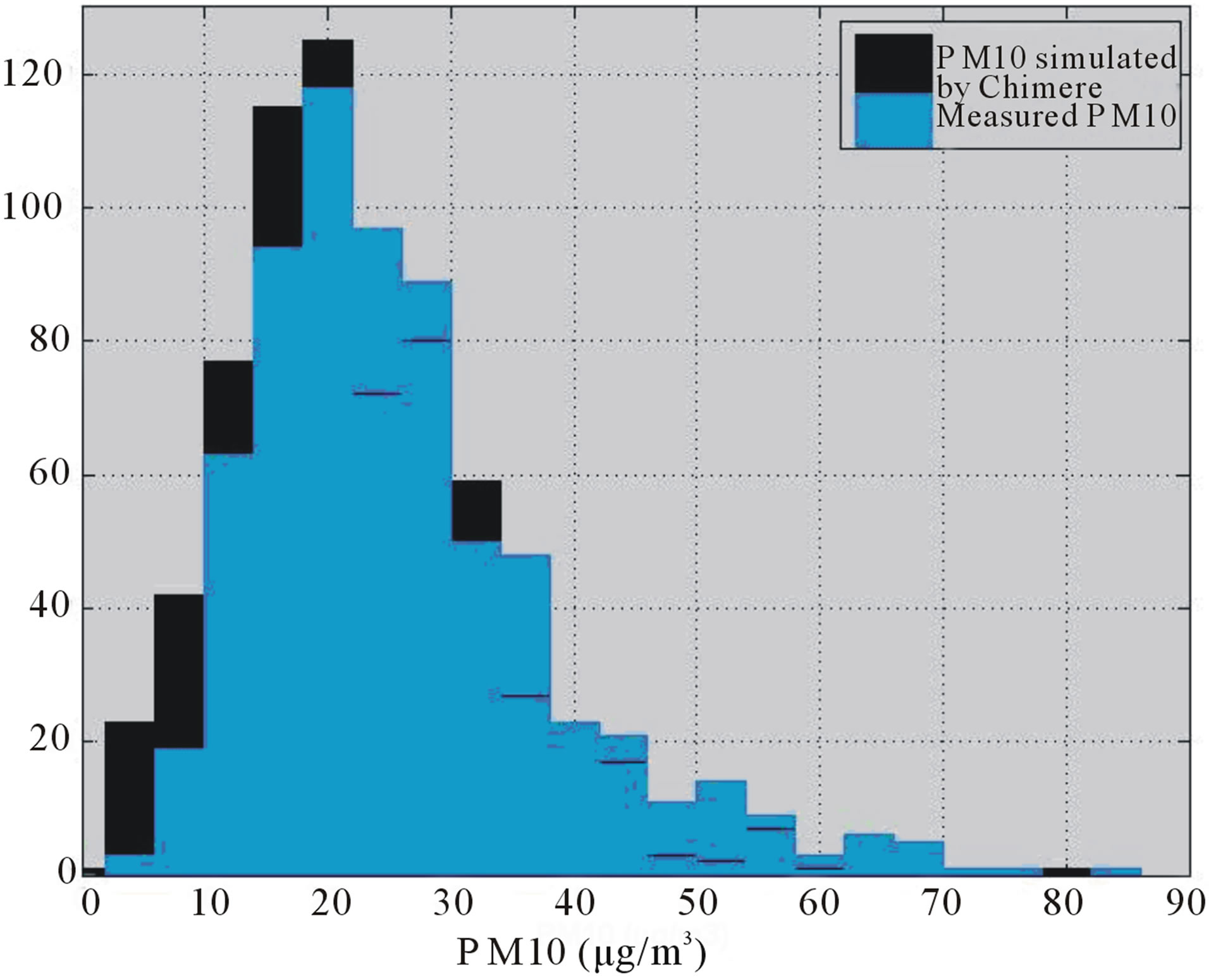
Figure 9. Comparisons between histograms of hourly measured (PM10)Obs and simulated by CHIMERE.
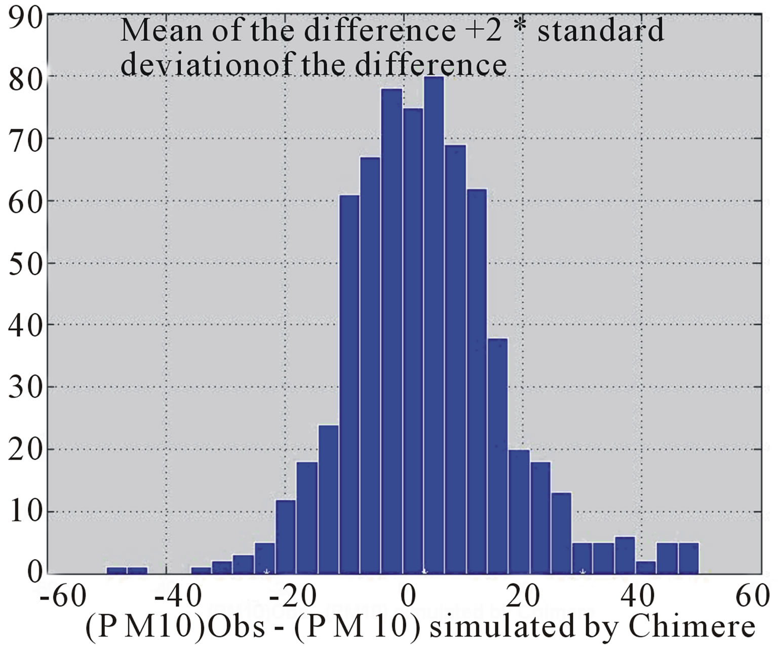
Figure 10. Histogram of the difference (μg/m3) between the PM10-Obs and the PM10 simulated by CHIMERE.
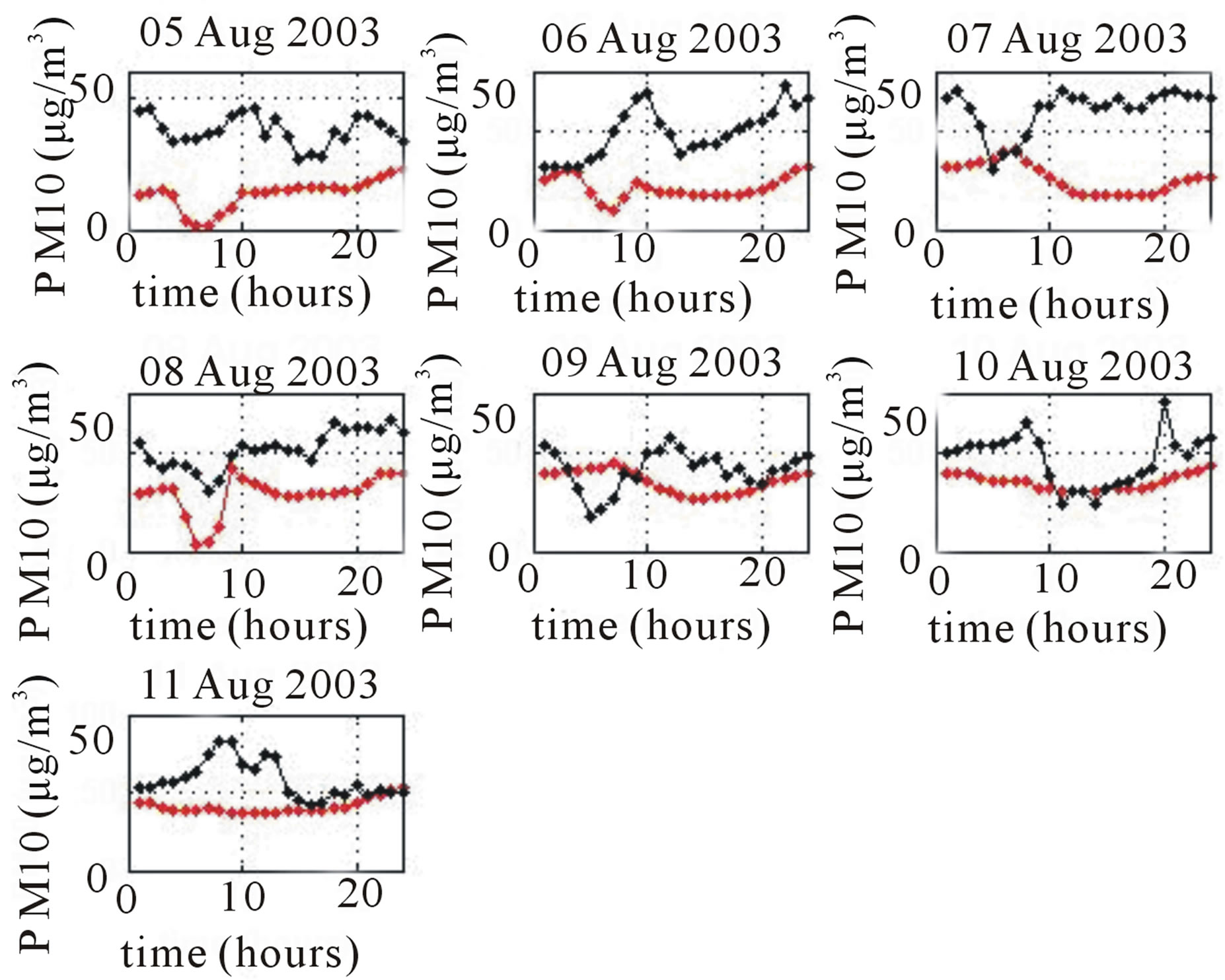
Figure 11. Time-series of the daily PM10 mass concentration from 5 to 11 August 2003. A hourly measurements (in black); b CHIMERE output (in red). Most of the PM10-Obs concentrations are over the 40 µg/m3 threshold, whereas the CHIMERE values hardly ever exceed that threshold.
were constructed from the output of the meteorological numerical model MM5, which was also the dynamical forcing for CHIMERE. Figure 12 shows the mean PM10 concentration profiles for the studied period provided by CHIMERE for the lower layers of the atmosphere for each weather type. We have also added the mean PM10 concentration measurements (red stars in Figure 12). The CHIMERE profiles and the measured PM10 are different for the different weather types. The CHIMERE model gives a PM10 concentration in good agreement with the PM10 measured at the ground stations for weather types 2 - 4 and 8. The mean CHIMERE profile giving a PM10 concentration at the surface that differs the most from the PM10 concentration measured at ground station belongs to weather type 7. This case corresponds to the heat wave of August 2003 and it is a weather type for which an alert threshold can be dispatched.
5.4. Case Study: Analysis of the Pollution Events of 5 to 12 August 2003
Weather type 7 is associated with high AOT and PM10 values and a strong pollution index (index 4). The discrepancy between the measured PM10 and the CHIMERE PM10 values (Figure 11) suggests that the CHIMERE model underestimates the pollution events.
Examining the time-series of PM10 concentration and the associated weather types, we find that 25% of the data belonging to weather type 7 were measured during the first two weeks of August 2003. This period was characterized by an exceptional heat wave associated with persistent high pressure conditions characterized by very high temperatures ([19]). Figure 13 presents a sketch of the time-series for the summer of 2003. During that period (of weather type 7), pollution level was very strong. Indeed the meteorological conditions were favourable to the development of a large-scale photo chemical pollution episode, ([11]). The stagnation of the air mass also led to the accumulation of primary emitted particulate matter (PM) and the development of secondary aerosols. Modelling such a pollution episode is a challenging problem because models have to deal with an exceptional environment for which their parameterizations and input are not necessarily appropriate. For instance, the formulation in classical models of dry gaseous deposition or biogenic emissions does not generally account for the exceptional deficit in soil water.
During the August 2003 pollution event, PM10 measurements overshot the 40 µg/m3 concentration threshold for six days at Lille, while the CHIMERE concentrations reached that value one day only (Figure 11). The 40 µg/m3 threshold standard is a particular value which deserves a deeper analysis.
Figure 14 shows the time-series of the PM1n0 co cen-
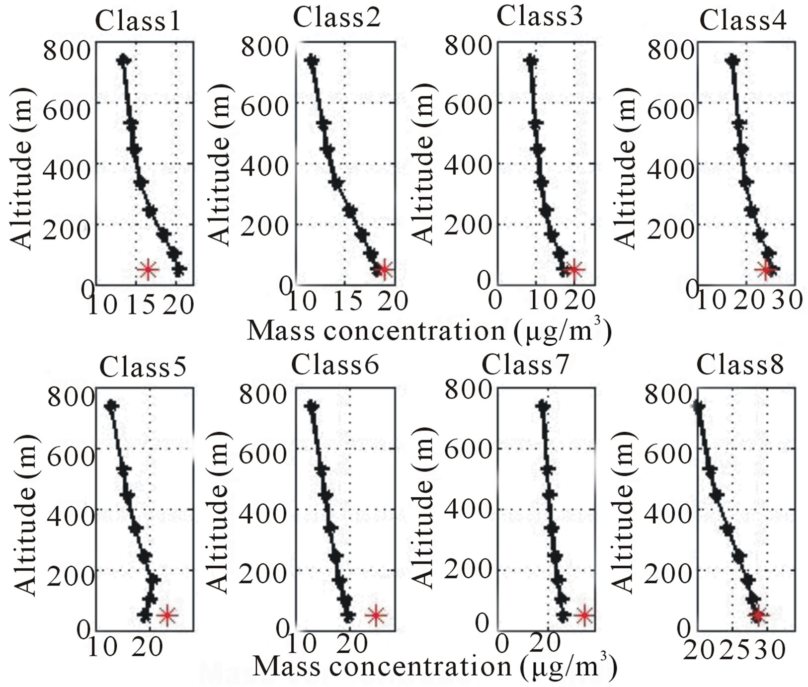
Figure 12. Vertical profiles of mean CHIMERE PM10 values and of mean ground-level PM10 measurements (red stars) for the eight weather types.
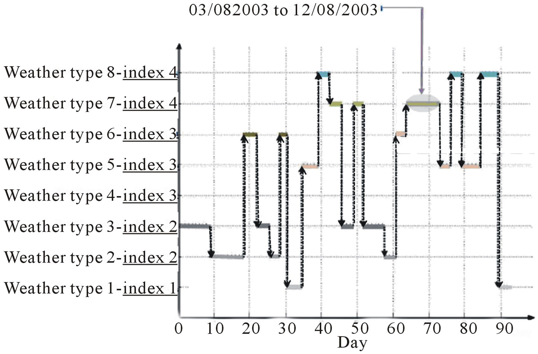
Figure 13. Time-series of the weather types and the associated pollution indices during the 2003 summer.
tration retrieved by inverting AOT observations, those measured by the surface stations with TEOM and those estimated by the CHIMERE forecast for the strong pollution event of the first two weeks of August 2003. It is clear that the AOT inversion (in green in Figure 14) gives a good retrieval with a good accuracy. The neuronal inversion of AOT measurements presented above was able to detect the August 2003 pollution event. This method, which is based on a classification of the meteorological situations into different weather types, could be used for activating pollution alerts.
To better determine the differences between PM10- Obs and CHIMERE PM10 we have tried to relate the (PM10-Obs - PM10 CHIMERE) to PM10-Obs.
The result, (shown in Figure 15), is interesting since it shows a significant increase of the difference with the PM10-Obs level though the scatter is large.
This statistical relationship says nothing else that the model deviation (difference between observation and model) increases linearly as when the observed PM10 increase. This relationship, if it is statistically significant could at least help to retrieve a PM10 model forecast.
It seems at this point convenient to compare the regional CHIMERE PM10 forecast to the local PM10 observations at the 5 sites of the Lille region, see Figure 1. This analysis gives insight into local deviations and helps to see if they follow the same kind of relationship which indicates (by linear correlation construction) the level of correlation between observations and model.
The regression results in Table 5 show different information items:
1) From East to West the correlation coefficients increase.
2) The three sites of (Faidherbe, Marq-Barouel and Lomme) have equivalent relatively large correlation coefficients and equivalent regression coefficients which show a homogeneity in the deviation behaviour.
3) The two eastern sites of Five and Tourcoing have a correlation coefficient close to the limit of the signifi-
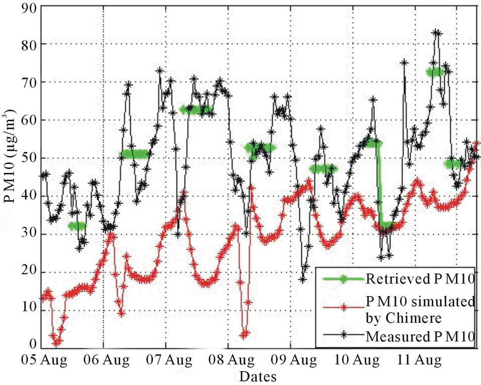
Figure 14. Time-series (for August 2003) of PM10-Obs, CHIMERE PM10 output, and AOT retrieved PM10.
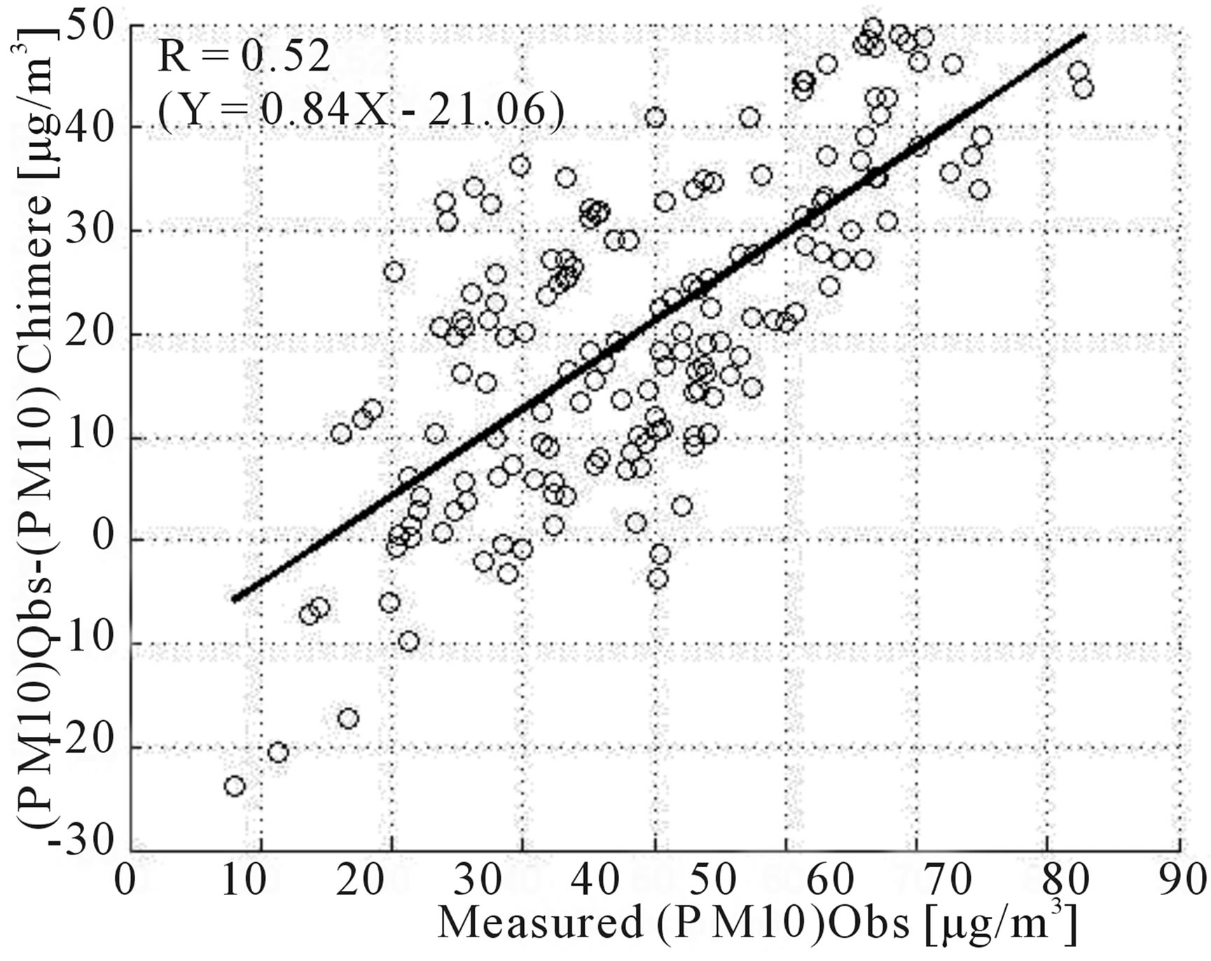
Figure 15. Scatter plot between deviations (differences between PM10 Obs-CHIMERE PM10) and PM10 Obs (measurred PM10).
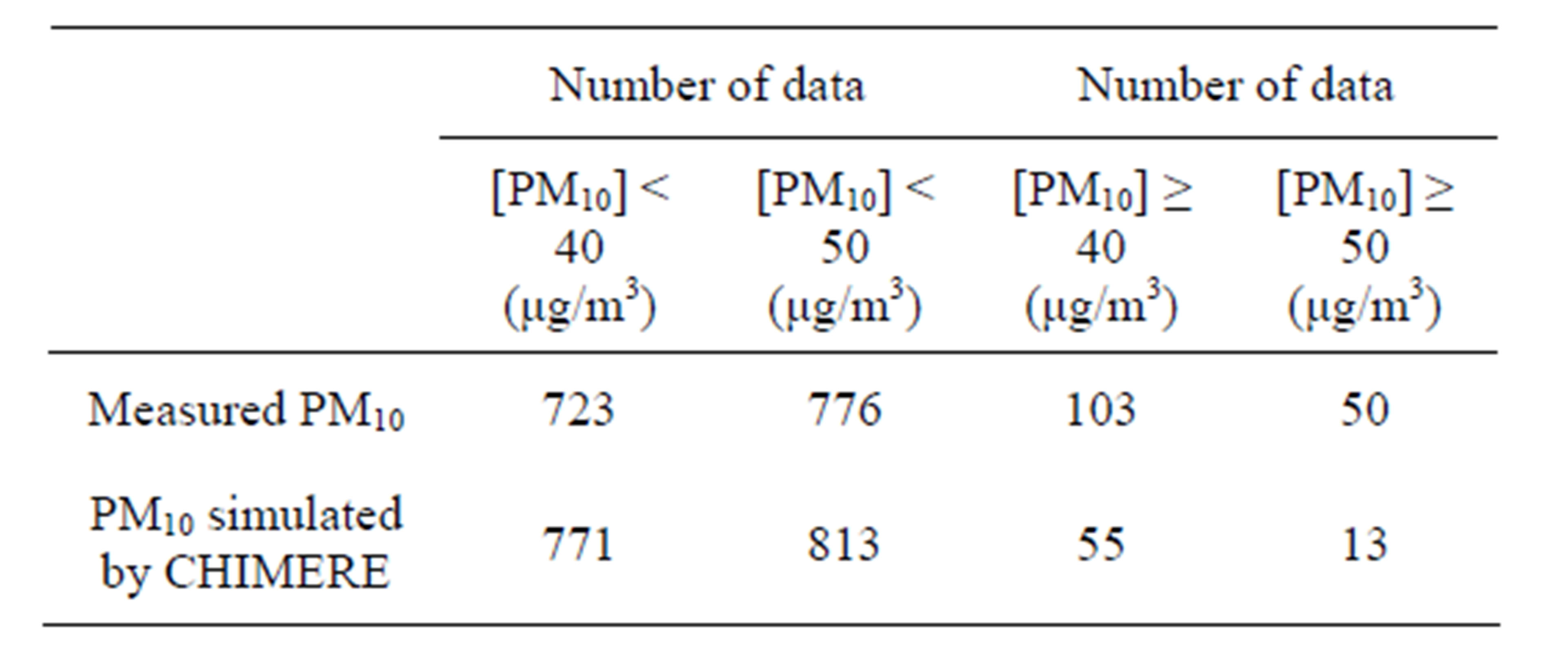
Table 4. Number of PM10 concentration values over the legal limit for the 836 hourly PM10-Obs and PM10 simulated by CHIMERE.
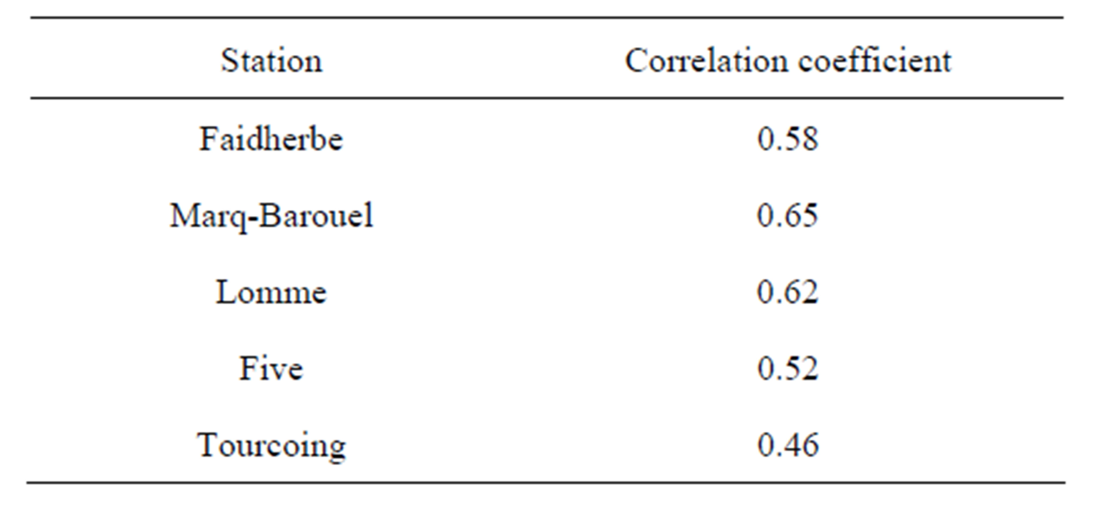
Table 5. Correlation coefficients between observations and deviations (differences between observations and model estimations).
cance and their regression coefficients are of the same order and very different from the three western sites.
This suggests a PM10 model noise different from west to east probably related to PM10 sources and a priori not included in the CHIMERE model. These behaviour differences cannot be associated with advection processes, since for class 7 the wind speed is very small. Lacunar information about PM10 sources or an imperfect knowledge of secondary aerosols is probably obvious. This aspect of imperfect knowledge of “urban pollution noise” has been evocated in model comparisons by [20]. They have indeed undertaken a classification into urban and suburban sites suitable for comparing models scores at representative sites.
Since the MM5 model (as most of meteorological models) is able to forecast meteorological situations with a very good quality up to five days, we can expect that weather types and consequently pollution indices can also be forecasted with a good skill. These pollution indices can be combined with AOT measured the previous days to infer an estimate of a forecasted PM10 and then an alert threshold. This simple forecasted PM10, which is easy to obtain could be combined with a more sophisticated CHIMERE PM10 forecast to deliver a confident forecast index with a probability occurrence. Moreover this type of analysis could help to precisely understand the physical processes occurring in the lower part of the boundary layer, which drive particles and chemistry profiles and their height variation during a specific experiment. This understanding could help to improve atmospheric chemical models. It can be also an alternative or a complement to the [20] classification to minimize bias in chemical forecast models.
6. Conclusions
This paper presents a method for retrieving PM10 concentration from AOT measurements done in the Lille region (France) with a sun photometer. We analyzed the summer time periods of the years 2003-2007. We gathered 836 AOT measurements collocated with PM10 measured by a microbalance (TEOM) at five ground stations around Lille. As PM10 concentration strongly depends on meteorological variables, we first clustered the meteorological situations in a number of classes (weather types) for which the AOT and PM10 relationship is expected to be simplified. A fine clustering of the hourly meteorological situations (vertical profiles of temperature, zonal and meridional wind components) was first done by using a self-organizing map (SOM) of 10 × 10 neurons. SOM was trained on 11,040 meteorological situations provided by the MM5 model. The large number of groups (100) provided by SOM allowed us to represent the large variety of meteorological situations, but prevented from synthesizing some geophysical information embedded in the Learning Set. We decided to aggregate this large number of subsets into a smaller number of types based on the similarities of the subsets. We thus extracted a few pertinent situation types from the subsets by clustering groups having similar statistical properties expecting that the types can be associated with geophysical characteristics. For that we used a hierarchical ascending classification (HAC) and clustered the groups into eight weather types having well defined properties in terms of meteorological variables. Since the meteorological situations are similar in each class, their effect on the retrieval procedure has been removed at first order at least. We then modelled the AOT-PM10 relationship for each weather type with a second SOM map, whose input are AOT and also the meteorological parameters taking into the second order effect. We then developed an iterative retrieval procedure. The eight AOT-PM10 relationships compared well with the PM10 measured at five ground stations around Lille, thus demonstrating the interest in the decomposition into weather types. Careful inspection of the weather types showed that each weather type corresponds to a well defined pollution index. The decomposition of the meteorological situations into weather types also allowed us to detect the occurrence of a strong pollution event, with a sufficiently high level of probability, from the dynamical model output only. By comparing the measured PM10 values to those produced by the CHIMERE model, we found that, for most of the weather types, CHIMERE PM10 values agree with the measured PM10. The marked discrepancy between the two PM10 estimations for weather type 7 significantly corresponded to a strong pollution event in August 2003 associated with a heat wave. While the AOT and the surface PM10 measurements were in good agreement, the CHIMERE output used in this work, did not easily detect this strong pollution event, owing to its underestimation of the PM10 values which can probably be explained by an inadequate emission cadastre. Therefore we suggest associating PM10 CHIMERE forecast with forecast using the dynamical model as MM5 and our method.
Prospectively, the statistical method we dealt, relating AOT to PM10 can be easily applied to monitor strong pollution events by using satellite radiometers. A major advantage of these satellite remote-sensing methods is that they can be practically applied everywhere (though geographical calibration might be necessary in some places) to construct spatial long pollution time-series. Such adequate satellite sensors already exist. The main drawback is that they can only operate on days without heavy cloud coverage. The clustering into weather types also proved to be an efficient tool for analyzing complex phenomena that depend on meteorological variables; it can also be used as a method to understand and analyze the errors made by chemical models and try to improve them. Our method also presents a good operational interest for forecasting pollution events.
7. Acknowledgements
We thank L. Menut for fruitful discussions. We are grateful for the support we received from R. Santer and the ADEME agency (“Agence de l’Environnement et de la Maitrisse de l’Energie”). We thank the INERIS agency for providing the CHIMERE and MM5 model output database, P. Goloub principal investigator of the Aeronet nload site of “Lille”, for their effort in establishing and maintaining the site. We also thank ATMO France (Fé- dération des Associations Agréées de Surveillance de la qualité de l’Air) for providing the database of direct measurements of mass concentration at the Lille stations.
REFERENCES
- Y. J. Kaufman, R. S. Fraser and R. A. Ferrare, “Satellite Remote Sensing of Large Scale Air Pollution Method,” Journal of Geophysical Research, Vol. 95, No. D7, 1990, pp. 9895-9909. http://dx.doi.org/10.1029/JD095iD07p09895
- A. Van Donkelaar, R. V. Martin and R. J. Park, “Estimating Ground-Level PM2.5 Using Aerosol Optical Depth Determined from Satellite Remote Sensing,” Journal of Geophysical Research, Vol. 111, No. D21201, 2006.
- D. A. Chu, Y. J. Kaufman, et al., “Global Monitoring of Air Pollution over Land from the Earth Observing System-Terra Moderate Imaging Spectroradiometer (MODIS),” Journal of Geophysical Research, Vol. 108, No. D21, 2003, p. 4661. http://dx.doi.org/10.1029/2002JD003179
- H. Yahi, R. Santer, A. Weill, M. Crepon and S. Thiria, “Exploratory Study for Estimating Atmospheric Low Level Particle Pollution Based on Vertical Integrated Optical Measurements,” Atmospheric Environment, 2011, p. 448.
- B. Pelletier, R. Santer and J. Vidot, “Retrieving of Particulate Matter from Optical Measurements: A Semiparametric Approach,” Journal of Geophysical Research, Vol. 112, No. D06208, 2007.
- Y. Liu, J. R. Key, R. A. Frey, S. A. Ackerman and W. P. Menzel, “Night Time Polar Cloud Detection with MODIS,” Remote Sensing Environment, Vol. 92, No. 2, 2004, pp. 181-194.
- H. Van Loon, G. A. Meehl and R. Milliff, “The Southern Oscillation in the Early 1990s,” Geophysical Research Letters, Vol. 30, No. 9, 2003, p. 1478. http://dx.doi.org/10.1029/2002GL016307
- J. L. Pearce, J. Beringer, N. Nicholls, R. J. Hyndman, P. Uotila and N. J. Tapper, “Investigating the Influence of Synoptic-Scale Meteorology on Air Quality Using SelfOrga-Nizing Maps and Generalized Additive Modelling,” Atmospheric Environment, Vol. 45, 2010, pp. 128-136.
- H. Patasnick and E. G. Rupprecht, “Continuous PM10 Measurement Using the Tapered Element Oscillating Microbalance,” Journal of the Air & Waste Management Association, Vol. 41, No. 8, 1991, pp. 1079-1083.
- B. N. Holben, T. F. Eck, et al., “AERONET-A Federated Instrument Network and Data Archive for Aerosol Characterisation,” Remote Sensing Environment, Vol. 66, No. 1, 1998, p. 1-16. http://dx.doi.org/10.1016/S0034-4257(98)00031-5
- R. Vautard, “Multiple Weather Regimes over the North Atlantic: Analysis of Precursors and Successors-Mon,” Weather Reviews, Vol. 118, 1990, pp. 2056-2081. http://dx.doi.org/10.1175/1520-0493(1990)118<2056:MWROTN>2.0.CO;2
- B. Bessagnet, A. Hodzic, R. Vautard, M. Beekmann, S. Cheinet, C. Honoré, C. Liousse and L. Rouil, “Aerosol Modeling with CHIMERE-Preliminary Evaluation at the Continental Scale,” Atmospheric Environment, Vol. 38, 2004, pp. 2803-2817. http://dx.doi.org/10.1016/j.atmosenv.2004.02.034
- B. Bessagnet, L. Menut, G. Aymoz, H. Chepfer and R. Vautard, “Modeling Dust Emissions and Transport within Europe: The Ukraine March 2007 Event,” Journal of Geophysical Research, Vol. 113, No. D15, 2008. http://dx.doi.org/10.1029/2007JD009541
- T. Kohonen, “Self-Organizing Maps,” 3rd Edition, Springer-Verlag, Berlin, Heidelberg, New York, 2001, 501 p. http://dx.doi.org/10.1007/978-3-642-56927-2
- A. K. Jain and R. C. Dubes, “Algorithms for Clustering Data,” Prentice-Hall, Englewood Cliffs, 1988.
- A. Hodzic, R. Vautard, B. Bessagnet, M. Lattuati and F. Moreto, “Long-Term Urban Aerosol Simulation 413 versus Routine Particulate Matter Observations,” Atmospheric Environment, Vol. 39, No. 32, 2005, pp. 5851-5864. http://dx.doi.org/10.1016/j.atmosenv.2005.06.032
- G. Allen and R. Ress, “Evaluation of the TEOM Method for Measurement of Ambient Particulate Mass in Urban Areas,” Journal of the Air & Waste Management Association, Vol. 47, No. 6, 1998, pp. 682-689. http://dx.doi.org/10.1080/10473289.1997.10463923
- C. Seigneur, “Current Status of Air Quality Models for Particulate Matter,” Air and Waste Management Association, Vol. 51, No. 11, 2001, pp. 1508-1521. http://dx.doi.org/10.1080/10473289.2001.10464383
- I. Rasool, M. Baldi, K. Wolter, T. N. Chase, J. Otterman and R. A. Pielke, “August 2003 Heat Wave in Western Europe, An Analysis and Perspectives, European Meterological Society (EMS),” 4th Annual Meeting—Part and Partner: 5th Conference on Applied Climatology (ECAC), Nice, 26-30 September 2004.
- M. Joly and V.-H. Peuch, “Objective Classification of Air Quality Monitoring Sites over Europe,” Atmospheric Environment, Vol. 47, 2012, pp. 111-123. http://dx.doi.org/10.1016/j.atmosenv.2011.11.025
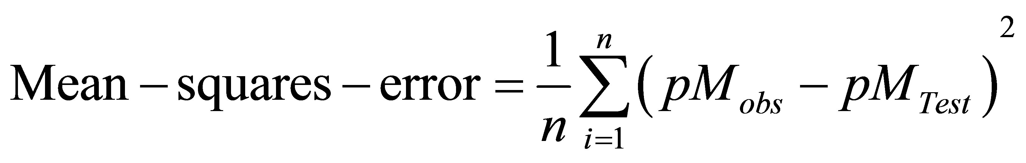
Annex 1
The mean squared error defined as
 the mean relative error defined as
 .
.