ABSTRACT

The counterparty risk issue has become increasingly important in the world of finance. This risk is defined as the loss due to the counterparty default. The regulator uses the Credit Value Adjustment (CVA) to measure this risk. However, there is the independency assumption between the default and the exposure behind the CVA computation and it is not verified on the financial market. This paper presents two mathematical models for the assessment and the quantification of the counterparty risk without this assumption. This kind of risk is known as Wrong Way Risk (WWR). This study focuses on three approaches: empirical, copula and mixed model. The first one is based on the hazard rate modelling to express the correlation between the probability of default and the exposure. The second one is about calculating the WWR effect using copulas. The last one is a combination of both. There is another assumption that makes easier the CVA computation: The constant of the loss given default (LGD). As we know this assumption is not verified because the LGD could be deterministic or stochastic. Otherwise, it could lead to a correlation effect between the LGD, the exposure and the default, and we then obtain a Global Wrong Way Risk (GWWR). Indeed, we propose a model allowing the CVA quantification without these assumptions.

Keywords:

Counterparty Risk, Credit Value Adjustment, Wrong Way Risk, Copulas

1. Introduction

The credit value adjustment (CVA) computation is based on the independency assumption between the exposure and the default. However,this assumption is not verified on the market, and we although have correlation between the probability of default (PD) and the exposure at default (EAD). Therefore, we get two types of this effect: The Wrong Way Risk (WWR) when the correlation is positive and the Right Way Risk (RWR) when the correlation in this case is negative. There is another effect appears when the LGD becomes random and also depends on the default. Indeed, this could generate a correlation between the three variables that make the CVA assessment. In this case, we could call this effect as the Global Wrong Way Risk (GWWR). First, we will focus on the WWR effect and we make the difference between two kinds:

・ The systemic WWR: this kind arises at the moment where the dependency between the exposure and the default is due to a macroeconomic factor. In this case, this factor increases the EAD and the PD. If we take a put on the CAC40 index with some bank like Société Général (SG) as the issuer, then the CAC40 spot impacts both of the exposure and the counterparty rating. In fact, this index is a systemic factor in the French market and the SG is a part of the CAC40 composition.

・ The specific WWR: on the other hand, this kind comes from a specific factor. For example, we get this effect when we have a put on the stock of the issuer as underlying.

There are several models allowing the CVA computation with the WWR component. We present some of these approaches:

・ The Basel model¹ ( Basel Committee on Banking Supervision, 2010 ): this approach is the most straightforward one to add the correlation effect and it is used by the Basel committee to add the WWR effect in the counterparty credit risk (CCR) charge. It is based on the multiplier coefficient, to explain this effect. The exposure at default is given by the formula bellow:

With represents the expected effective positive exposure.

We have by default, whatever, banks could have values above 1.2. Other institutions use values bigger than the default one. The coefficient value is appreciated, on one hand, by the name concentration and that also means the portfolio granularity by counterparties. On the other hand, we have the correlation effects between assets of the same counterparty. The Basel II accords do not give details to manage the WWR. However, Basel III brings more precision to manage this kind of risk, focusing on three aspects:

Ø Implementation of a detailed process to manage the WWR.

Ø Advising banks to put more provision to cover the counterparty risk.

Ø Explication of the approach to manage transactions containing the specific WWR.

The implementation of this model remains easy and could be automatically integrated to the existent model, but it has two drawbacks:

Ø It does not give the contribution part of the WWR.

Ø It consumes more capital requirement to cover the counterparty risk, because the standard approach is designed for the worst case.

・ The empirical approach: this approach uses the hazard rate according to the exposure. Indeed, the relation between these two quantities allows getting the diffusion of the PD, and then it could explain the correlation with the exposure. The WWR modeling progresses into three steps:

Ø The choice of the function that gives the relation between the hazard rate and the exposure. The diffusion calculation is performed for each time step:

With represents the exposure. Hull and White² ( Hull & White 2012 ) suggests an exponential function to implement this method.

Ø The PD computation is done using the below formula:

Ø The computation of the CVA WWR using the Monte Carlo simulation. This step is deduced directly from the exposure diffusion.

This approach allows a straight integration within the existent CVA model. In fact, it replaces the computed PDs under the independency assumption with the new one using the dependency between the default and the exposure.

・ The copula model: This approach is based on copulas to explain the relation between the default variable and the exposure. Rosen and Saunders³ ( Rosen & Saunders 2012 ) use the Vasicek model to make this dependency. They introduced the Gaussian copula to compute the expected exposure without the independency assumption. Their model is implemented in three steps:

Ø The default is written as a latent variable and it is divided in two components. The first part represents the specific risk, and the second part is the systemic risk:

where and are two independent random variables and they follow a Gaussian distribution. The counterparty is deemed in default when is lower than. The conditional probability of default regarding to the systemic variable is expressed as:

With represents the unconditional probability of default.

Ø Future exposures are mapped to a market variable that also follows a Gaussian distribution. The relation between this variable and the exposure is:

With represents the distribution function of exposure and it is uniform.

Ø This model supposes that the two variables and are linked to a bivariate joint distribution. This relation is expressed under a Gaussian copula with the correlation between both of variables. Bocker and Brunnbauer⁴ ( Bocker & Brunnbauer, 2014 ) generalized this concept to use others copulas. This approach allows a straight integration within the existent CVA model.

The next section will be devoted to the WWR mathematical modeling using a mixed model. Indeed, we will use the empirical model to build the diffusion of PDs, and then we will explain the relation between the default and the exposure under copulas model.

2. Mathematical Modeling of the WWR

The Credit Value Adjustment (CVA) is defined by the difference between the portfolio value without the counterparty default and with this component. The CVA could be written as:

where represents the risk free portfolio value, and is the portfolio value taking in consideration the counterparty default.

Using this, we find the following formula:

With is the default time, , represents the discount factor, and defines the Loss Given Default that we deem constant in this section.

We also can write:

where, and defines the distribution of the default.

First, we begin by modeling the probability of default using the empirical model. For this, we introduce the hazard rate concept that measures the counterparty default occurrence. Giving the assumption that the default frequency follows the Poisson density, we get the formula below:

The relation between the, and the exposure is written as:

With is defined positive since.

This function should also verify the following relation under the assumption that the hazard rates curve is flat:

With defines the arithmetic average of simulated values until the date, and is the market spread with the maturity of.

We deem the following function of the hazard rate:

where is a function of time and determines the correlation between and, and is a function of time.

We can find the stochastic derivative equation (SDE) of the hazard rate by applying the Itô’s lemma on the, and we get:

With, defines the volatility of and repre- sents the Brownian motion under the risk neutral measure.

We conclude that the hazard rate follows a log-normal distribution with parameters below:

In our case, we more interest about the distribution of the time integration of the. If we take the following approximation and by using the Fenton-Wilkinson⁵ ( Fenton, 1960 ) approach, this quantity then follows a log-normal distribution with parameters below:

With,

It also supposes that are independent. We get the following result by applying the Laplace transform approximation:

If, then

The calibration is made in each time of the Monte Carlo simulation. Indeed, we minimize the distance between the PD model and the PD market basing on spreads. So, we need to do this process times using the discretization form of the hazard rate:

where and represent the j^th simulation of the exposure and the hazard rate.

The Appropriate parameters are those who minimize the following quantity:

where is the Monte Carlo number of simulation, is the number of steps time, and represents the spread with maturity.

Finally, when the parameters are computed, then the hazard rates are built sequentially at each time step. The next step allows to define the relation between the exposure and the probability of default distribution. Therefore, we use the copulas to get this relation, and we take the following definitions:

・ The value of the discount exposure at time follows a distribution with her density function.

・ The default time of the counterparty is a random variable and we note his distribution function by and with the density.

・ The joint distribution of and is defined by:

where indicates the bivariate copula and we suppose is twice continuously differentiable function. The density function is written as:

The expected positive exposure (EPE) is equal to:

With

We also have:

We then replace the value of the conditional density in the formula to get the following result:

By applying the strong law of large number, we obtain the following approximation of the EPE:

It remains one issue to complete those calculations; we are talking about the estimation of the correlation between the exposure and the probability of default. In fact, it is the requirement parameter to compute. We suggest two approaches to do this estimation:

・ The first one uses the Spearman⁶ ( Daniel, 1990 ) correlation who is defined as:

where presents the ranks difference between the exposure and the probability of default, and is the number of observations. We compute this correlation at each time step and we use the result of the hazard rate

diffusion for this. Finally, we can estimate the correlation by.

・ The second one is based on the minimization of the difference between the simulated survival probabilities at time using the hazard rate model and the copula at each time step:

We then can estimate the correlation by.

We have now all components to complete the CVA computation with the WWR effect. It remains to calculate all and apply the trapezoid integration method regarding to the PDs to get the value. The implementation of the mixed model approach will be done on the CAC40 European put option. We will use the HESTON⁷ ( Heston, 1993 ) model to compute the put price that is based on the stochastic volatility. We then take the following assumptions:

・ The Loss Given Default is constant and equal to 60%.

・ The discretization of time space is done on 100 steps.

・ The dividends are equals to 0.

・ The credit spread of the counterparty is constant and equal to 0.8%.

・ The CAC40 put strike value is 4350.

・ The Credit Support Annex (CSA) contains a Margin Call with 10 days as Margin Dates and the calculation will be done with and without collateral.

The value of the correlation between exposures and defaults using Spearman is equal to. The Figure 1 shows the evolution of the EPE regarding to the PD with and without collateral using the Gaussian copula:

We conclude that the EPE increases with the WWR effect and the CVA will also have the same behavior. The Figure 2 displays this effect:

The WWR increases the CVA quantity with 30%, and that proves its importance and impact on the counterparty risk measurement. The Table 1 summarizes these results.

3. The Global Wrong Way Risk (GWWR)

As we saw in the last section, the compute of the CVA supposes that the LGD is constant. Furthermore, this assumption leads to the independency of this variable to the default. Nevertheless, the LGD depends to the default and automatically to the exposure, because the WWR proves that there is a dependency between the exposure and the default. We choose the word “Global” because we study the dependency between the three components that allow the calculation of the CVA. In order to model the Global Wrong Way Risk, we suggest two approaches:

・ The first approach is based on the building of a relation between the LGD and the exposure, and also, the definition of the relation between the exposure and the default. We use the same notation in the last section and we link the LGD with the exposure through the below function:

With.

We then replace in the CVA formula:

There is two ways to compute this expectation, on one hand; we can make it with empirical approach. We define the relation below:

With is defined positive since.

We so get the following result:

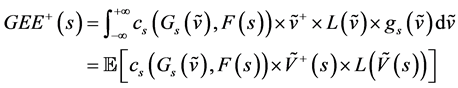
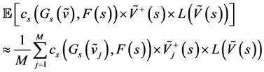
By applying the strong law of large number, we have at each step of time the approximation of the Global expected positive exposure (GEPE):

Using the trapezoid method for calculation the integral, we get:

On the second hand, we can use the copula approach. Given the definitions in the last section, we have:

Knowing that,

We get the following result:

By applying the strong law of large number, we obtain the following approximation of the GEPE:

We compute this quantity at each time step, and then we use the trapezoid method to compute the GWWR CVA.

The implementation of this approach needs to choose the link function between the LGD and the exposure. We then suggest the following function:

where

The calibration of the LGD model could be done by defining the maximum and the minimum of the LGD. If we note respectively and the lower and the upper bound, we thus obtain:

In our case, we take and. We get the following values of

The Figure 3 displays the evolution of the GEPE regarding to the PD with and without collateral using the Gaussian copula:

We deduce that the GEPE increases with the GWWR effect and the CVA will also have the same behavior. The GWWR grows the CVA quantity with 100%, and that proves its importance and impact on the counterparty risk measurement. The Table 2 summarizes these results:

The Figure 4 shows this effect:

・ The second approach is built around the approximation of the difference between the classical CVA, and the other one without any assumptions using a close formula. We suppose that the default is driven via a systemic factor

and the default arises at time when the reaches some level:

We can write the CVA under to the independency assumption as:

With

We note the Global Wrong Way Risk CVA by and we define the following function:

For, we have.

We define the following quantities:

Under the assumption of independency of,. Using these notations, the Global Wrong Way Adjustment (GWWA) is defined as:

For a.

By applying the Taylor expansion on with second order according to the and by replacing the, we get:

By computing the first and the second derivative terms, we find the following results⁸ ( Gourieroux, Laurent, & Scaillet, 2000 ):

where represents the density function of the systemic factor.

We then find the result bellow⁹ ( Slime, 2016 ):

We need to define a model for computing this quantity, and we then chose the CreditRisk+¹⁰ ( Credit Suisse Financial Products, 1997 ) model. This model supposes that where and we obtain the following relation:

Which represents the dependence factor between the counterparty and the systemic factor.

We also need to develop the derivative terms to complete the calculation, so we have:

and

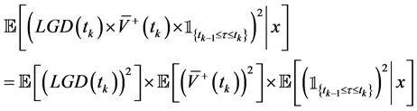
The CVA assumption is the independency between the LGD, the exposure and the default, and this allows us to compute the following term:

The second assumption of the CreditRisk+ model is that follows a Poisson distribution with as intensity. So, we deduce that:

We get the result bellow:

With

And

We conclude that:

Subtitling in the GWWA formula, we obtain:

If we note the classical CVA by:

Then we have: and

Finally, we get the following formula:

With

And

Under the assumption of, we obtain the simplified formula of GWWA:

Furthermore, the Global Wrong Way Risk CVA may be approximate using the formula bellow in the case of a symmetric distribution:

For non-symmetric distribution, we have:

As we know that the systemic factor follows the Gamma distribution, we could calibrate the factor using the Maximum Likelihood Estimation (MLE). We deem observation of and the likelihood function is defined by:

We then should compute the maximum of the logarithmic function:

It remains to develop the first and the second derivative. The calculation leads to the following results:

We use the Stirling approximation to resolve this equation:

We compute the estimator, we then get. This estimator must verify the second condition, and we obtain by computing the second derivative:

The Figure 5 and the Table 3 summarize the comparison between all approaches. The approximation of the GWWR using the adjustment has a tow strong advantage. The first one, it gives us a closed formula to compute the GWWR part. The second one, his implementation is straightforward and it

could be directly integrated on the existent framework.

We also conclude in the Figure 6 that the conditional default probability decreases within , and the GWWA follows the same effect. This makes sense with the definition of the GWWR. Indeed, the exposure should also decrease regarding to the conditional PD, and the GWWA must be reduced.

4. Conclusion

This paper was dedicated to the models allowing, on one hand, the quantifying of the Wrong Way Risk. On the other hand, we also developed two methods to integrate the Loss Given Default correlation effect. First, we began by introducing the existent approaches that give us the measurement of the WWR effect when we observe the positive correlation between the exposure and the default. We proposed a new model that combines the empirical and the copulas model. We made implementation on the European CAC40 put, and we conclude that the CVA increases potentially with the WWR effect.

Then, we generalized the concept to deem the correlation effects between the three variables. So we added the LGD correlation effect, and we proposed two models in this way. The first one is based on the definition of the function that links the LGD with the default and we also used the copula to compute the conditional expectation exposure. The second one defines a close formula to compute the difference between the classical CVA and the other one without the independency assumption.

We implemented both of these models on the European CAC40 put, and we concluded that the GWWR is more important than the WWR in term of the CVA level. Furthermore, the GWWA allows a direct integration and computation of the GWWR and we can also apply this model to the WWR. However, both of models represent some weakness. The first one needs to define and calibrate the LGD model, and the integration of the existent model is not straightforward and will cost more time calculation. The second one remains an approximation of the GWWR and requests a calibration of the systemic factor. We tried to give a close formula to allow a direct integration on the existent CVA system, because the implementation arises one of most issues in the banking platform. By the way, we suggest getting more researching on the approaches that allow a straight integration.

Cite this paper

Slime, B. (2017). Modeling and Quantifying of the Global Wrong Way Risk. Journal of Financial Risk Management, 6, 231-246. https://doi.org10.4236/jfrm.2017.63017

References

NOTES

¹Basel Committee on Banking Supervision (2010), “Basel III: A Global Regulatory Framework for More Resilient Banks and Banking Systems”.

²J. Hull and A. White (2012), CVA and Wrong Way Risk, Financial Analysis Journal, 68, pp. 58-69.

³D. Rosen, and D. Saunders (2012), CVA Wrong Way Risk, Journal of Risk Management in Financial Institutions, 5(3) pp. 252-272.

⁴K. Bocker and M. Brunnbauer (2014), Path consistent Wrong Way Risk, Risk Magazine.

⁵Fenton L. (1960) the sum of lognormal probability distribution in scatter transmission system, IEEE trans. Communication Systems, Vol 8, pp. 56-57.

⁶Daniel, Wayne W. (1990). “Spearman rank correlation coefficient”. Applied Nonparametric Statistics (2nd ed.). Boston: PWS-Kent. pp. 358?365.

⁷Heston, S.L., (1993), A closed-form solution for options with stochastic volatility with applications to bond and currency options, Review of Financial Studies, Vol.6, No 2, pp. 327-343.

⁸C. Gourieroux, J.P. Laurent, O. Scaillet (2000), Sensitivity analysis of Values at Risk, Journal of Empirical Finance.

⁹Slime, B. (2016). Credit Name Concentration Risk: Granularity Adjustment Approximation. Journal of Financial Risk Management, 5, 246-263.

¹⁰Credit Suisse Financial Products (1997). Credit Risk+: A Credit Risk Management Framework. London, 1997.