American Journal of Climate Change
Vol.1 No.1(2012), Article ID:18072,13 pages DOI:10.4236/ajcc.2012.11001
The Impact of Climate Change on Crop Yields in Sub-Saharan Africa
Joint Program on the Science and Policy of Global Change, Massachusetts Institute of Technology, Cambridge, USA
Email: eblanc@mit.edu
Received February 8, 2012; revised March 4, 2012; accepted March 12, 2012
Keywords: Climate Change; Crop Yield; Error Correction Model
ABSTRACT
This study estimates of the impact of climate change on yields for the four most commonly grown crops (millet, maize, sorghum and cassava) in Sub-Saharan Africa (SSA). A panel data approach is used to relate yields to standard weather variables, such as temperature and precipitation, and sophisticated weather measures, such as evapotranspiration and the standardized precipitation index (SPI). The model is estimated using data for the period 1961-2002 for 37 countries. Crop yields through 2100 are predicted by combining estimates from the panel analysis with climate change predictions from general circulation models (GCMs). Each GCM is simulated under a range of greenhouse gas emissions (GHG) assumptions. Relative to a case without climate change, yield changes in 2100 are near zero for cassava and range from –19% to +6% for maize, from –38% to –13% for millet and from –47% to –7% for sorghum under alternative climate change scenarios.
1. Introduction
Climate change is an important environmental, social and economic issue. It threatens the achievement of Millennium Development Goals aimed at poverty and hunger reduction, health improvement and environmental sustainability [1]. Such issues are particularly important for Sub-Saharan Africa (SSA) where many people depend on agriculture for subsistence and incomes [2]. Agriculture, and especially crop growing, is heavily dependent on weather events in SSA, where 97% of agricultural land is rainfed [3]. The impact of climate change on crop yields is therefore a major concern in this region.
A large number of studies have investigated several aspects of the impact of climate change. Two main techniques are used to evaluate the effect of climate change on yields: 1) crop growth models and 2) regression analyses. Crop growth models are widely used and produce precise crop yield responses to weather events. In a seminal paper, Rosenzweig and Parry [4] provide a global assessment of climate change on world food supply and predict grain yield losses of up to 10% in several SSA countries between 1990 and 2080. However, crop growth models require daily weather data and are calibrated under experimental conditions.
Alternatively, regression analyses allow the quantification of weather changes on crop yields in an actual cropping context. Barrios et al. [5] estimate the impact of weather changes on agriculture net production index in SSA versus non-SSA countries. Among the few regression-based impact assessments of future climate change on crop yields in Africa, Ben Mohamed et al. [6] and Van Duivenbooden et al. [7] consider millet, cowpeas and groundnut in Niger. The most extensive assessment for SSA is provided by Schlenker and Lobell [8]. These authors predict median yield reductions ranging from 22% for maize to 8% for cassava when considering 16 climate change models for the mid-21st century.
Similarly to Schlenker and Lobell [8], this study estimates single output production functions for SSA in aggregate. Separate equations are estimated for the four most commonly grown crops in SSA (cassava, maize millet and sorghum) only. This study builds on existing literature in three ways. First, this study implements a more refined econometric analysis by appropriately treating non-stationarity data and using an estimator tailored to the specific attributes of the data. Second, in addition to standard temperature and precipitation variables, this study considers weather variables for evapotranspiration, standardized precipitation index (SPI), droughts and floods. Finally, by considering 20 climate change scenarios and allowing for technological changes, this study facilitates a comparison of predicted future yields under climate change and no climate change scenarios.
The article is divided into six further sections. Section 2 describes the production function specifications and the methodology employed. Section 3 presents the data used. Regressions results are presented and discussed in Section 4. Climate change predictions are described in Section 5. The predicted impact of climate change on yields for mid-2000 and late-2000 are presented in Section 6. Conclusion comments are presented in Section 7.
2. Modeling Framework
2.1. Production Function Specification
Traditionally, empirical studies have estimated the relationship between agricultural output and land, labor and capital inputs [9]. Land productivity in Africa, like in other regions, often differs within farms [10]. Farmers usually cultivate better soils first and then expand onto land of lesser quality, which implies that the marginal productivity of land is decreasing. Area harvested is therefore included in the production function to represent decreasing marginal productivity.
Labor is also a key determinant of agricultural production in Africa, as 89% of cultivated land is cropped manually [11]. In 1992, about 65% of SSA’s population was involved in agriculture [12]. However, as most of the labor input for African farms comes from family members, the level of labor input depends on family structures, in addition to the number of hours worked and work efficiency [10]. Furthermore, agricultural labor input requirements vary depending on the season, and labor characteristics such as education, health and farming experience determine agricultural yields through work capacity and the quality of crop management practices. As labor data are limited for SSA and population data are poor proxies for labor, this factor is not considered in the production function specification.
The level of mechanization also greatly influences agricultural efficiency [13]. However, capital requirements for traditional agriculture are low [14] and African agriculture relies mainly on non-mechanical power: animal power is used on 10% of cultivated land and mechanical machinery is used on only 1% of cultivated land [11]. Therefore, mechanization is also not considered.
Precipitation is also a major determinant of crop growth and yields in rainfed areas. The impact of water supply on crop yields is generally estimated using cumulative annual rainfall [15,16], or growing season rainfall [17]. Precipitation is generally found to have a positive impact on crop yields. Standardized precipitation is also used to represent precipitation when a large variety of climatic zones are considered. This measure is uninfluenced by scale effects as it calculates a standardized departure from the mean of a long-term trend [18]. The SPI proposed by McKee et al. [19] is calculated by first fitting a gamma probability density function to the frequency distribution of rainfall over the reference period. The probability density function is then used to determine the cumulative probability of a particular precipitation level for a chosen time scale. Finally, the calculation is transformed into a normal distribution with a mean of zero and a variance of one (~N(0,1)) to obtain SPI values expressed in standard deviations from the median. Negative SPI values indicate below normal rainfall and positive SPI values indicate above normal rainfall. Different time scales, ranging from 1 to 48 months, can be used to calculate the SPI. In this study, a 12 month (January to December) SPI is calculated. The period 1901-2002 is used as a reference period. The SPI is generally positively correlated with crop yields [20-22].
Using the SPI, it is possible to identify periods of drought [19] and floods [23]. In this study, droughts and floods start when the SPI reaches values of –1.5 and +1.5 respectively and ends when the index returns to a positive and negative value respectively. The SPI-based drought and flood spell indices have only recently been used in regression analyses [24-26].
The effect of average temperature on yields has been widely studied in econometric analyses, and generally has a negative effect on crop yields [20,27-30]. A more comprehensive indicator of weather conditions is provided by the evapotranspiration (ET) rate. ET is the combination of the loss of water from soils (by evaporation) and from crops (by transpiration). If rainfall and/or irrigation do not meet ET demand, a water stress occurs, which reduces crop yields [31]. Evapotranspiration is mainly used in regression analyses to represent crop water use [32,33]. There are several alternative ET measures. However, due to data limitations, only the reference evapotranspiration (ETo) rate can be calculated for this study. The Hargreaves equation [34] specifies ETo as:
 (1)
(1)
where Tavg, Tmax and Tmin are respectively mean, maximum and minimum temperature, and Ra represents extraterrestrial radiation and is calculated following Allen et al. [35].
Several crop yield determinants are not considered in this study. For instance, fertilizer use in SSA is low compared to the rest of the world, due mainly to market inefficiencies and low levels of liquidity held by farmers and high fertilizer price relatively to crop sale prices [36]. According to FAO [37], SSA’s fertilizer consumption is not expected to rise significantly in the next two decades. Irrigation is used in only 3% of the cultivated area in SSA and no change is expected [38]. This is partly because of unfavorable market and institutional situations but also a result of technical inapplicabilities due to poor soil quality and topography. Crop variety selection is also not considered, as farmers’ choices among cultivars is limited by seed supply and new seeds are not widely adopted in SSA [39]. Several other factors, such as crop management, weeds, pests, diseases and soil quality are not included in the analysis due to data limitations.
Quadratic terms for weather variables are included in specifications to account for non-linear weather effects on crop yields [40-42]. Interaction terms between weather variables are used to determine the potential effect of one weather variable given the effect of the other weather variable [43].
To avoid multicollinearity, two alternative specifications are considered for each crop. A first analysis, the T-P model, includes the most commonly used weather indicators, which are precipitation and temperature averages. The T-P model can be summarized as:
 (2)
(2)
where for each crop i at time t, Y represents yield, A area harvested, T temperature and P precipitation.
A second analysis evaluates the influence of ETo, SPI, drought and flood spells. In the ET-SPI regressions, a squared term for ETo is included and drought and flood dummies are used to represent the effect of extreme precipitation conditions. The ET-SPI model can be summarized as:
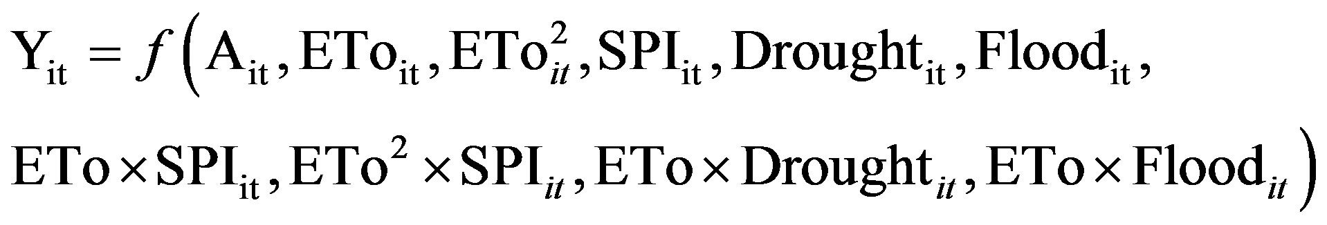 (3)
(3)
A third analysis considers the effect of CO2 concentration which is highly correlated with weather variables as changes in CO2 concentration drive changes in climate. Therefore, traditional weather variables are not included in specifications that include CO2 concentration. The CO2 model is specified as:
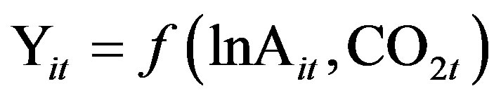 (4)
(4)
2.2. Methodology
A panel analysis is preferred as the sample size and quality of data are enhanced when combining a cross-section with time series. A panel analysis also allows one to control for time invariant unobservable factors that might affect the estimated coefficients, which is not possible in country specific studies. To control for omitted variables that vary over time but not across countries, time dummy variables are included for N-1 periods, when they are jointly significant.
One limitation of panel estimations is that parameters are assumed to be homogenous across countries. Generally, African countries share similar economic characteristics [44]. However, farming conditions may differ across countries as a variety of agricultural systems are observed in SSA [45]. Based on growth potential for different farming systems and their prevalence in each country, Diao et al. [46] distinguish countries with less favorable agricultural conditions (LFAC) and countries with more favorable agricultural conditions (non-LFAC)1. To account for potential parameter homogeneity across countries, a dummy variable equal to one for LFAC countries and zero for non-LFAC is created and interacted with the climatic variables in each specification.
The inclusion of quadratic and interaction terms results in the proliferation of similar terms, which can induce multicollinearity [47]. However, inappropriate inclusion of quadratic and interaction terms could produce incorrect nonlinearities and misleading relationships [48]. Therefore, for each model, a general to specific strategy is followed where the final specification is modified to exclude quadratic and/or interaction terms that are insignificant or have incorrect signs.
Regression studies generally include a time trend to represent the evolution of technologies. However, the estimation of the production function in first differences (without a time trend but with a constant) allows the impact of technology to be included without inducing multicollinearity.
Yield and area data are log-transformed to improve the distribution of variables, so the model estimates elasticities. Weather variables, on the other hand, are not log-transformed so as to produce semi-elasticities, which allow direct determination of the impact of, say, a 1˚C increase in temperature or a 10 mm increase in rainfall.
2.2.1. Unit Root Test
A panel series panels stationarity test such as Hadri’s [49] is not applicable as the current panel is unbalanced. Panel unit root tests such as Levin, Lin and Chu [50], Im, Pesaran and Shin [51] and Maddala and Wu [52] tests are not informative as, if the null hypothesis is rejected, they do not indicate which variables are non-stationary or the order of integration for each variable. Therefore, each series is tested for a unit root using the Elliott-RothenbergStock (ERS) time series test, which is a Dickey-Fuller generalized least square (DF-GLS) test using critical values from Elliott et al. [53]. This test is preferred to the augmented Dickey-Fuller test (ADF) because it has greater power and performs better in small samples.2 The ERS test has a null hypothesis of a unit root and an alternative hypothesis of stationarity. The test is first performed with a maximum lag length proposed by Schwert [56] and, in order to keep the sample as large as possible, the test is re-implemented with the maximum lag value reduced to the optimal lag length based on the SBIC criterion. As the data generating process is not known a priori, a constant and a time trend are included when implementing the test. Initially, the test is performed on variables in first difference to ensure that the series are not integrated of an order higher than one. All variables for which the ERS unit root test applied to first differences is rejected are tested for cointegration.
2.2.2. Cointegration Test
When using non-stationary variables, a spurious regression is of concern. Cointegration tests developed by Pedroni [57-59], McCoskey and Kao [60] and Kao [61] test for the presence of a unit root in the residuals. However, these tests assume cross-sectional independence which is unlikely in this study. A test developed by Westerlund [62] addresses the issue of cross-sectional dependence by bootstraping p-values. Westerlund’s approach tests the significance of the error correction (EC) term in an error correction model (ECM). If a cointegrating vector is found for the panel as a whole, an ECM is estimated.
2.2.3. Diagnostic Tests
The choice of estimator depends on the model to be estimated and the properties of the data. To determine the presence of cross-sectional correlation, the Breusch-Pagan test for cross-sectional independence described by Greene [63, p. 601] is performed. However, as this test is not applicable when the number of groups is greater than the number of years, a test developed by Pesaran [64] is used when the number of groups is large. To test for autocorrelation, a test proposed by Arellano and Bond [65] is applied. The presence of heteroskedasticity is tested using the panel heteroskedasticity test described by Greene [63], which produces a modified Wald statistic testing the null hypothesis of group wise homoskedasticity.
3. Data
FAOSTAT [66] provides data on area harvested (in hectares, Ha) and yields (in tonnes/Ha) aggregated at the national level from 1961 to 2002.3 Weather data extracted from the CRU TS 2.1 dataset [67] cover the period 1901-2002 and are available at the 0.5 × 0.5 degree resolution for all SSA. To consider only relevant weather data (e.g. avoid considering weather data for desert areas), grids are selected for crop growing areas using satellite-derived land cover data from Leff et al. [68]. Crop location data are provided at the 0.5 × 0.5 degree resolution, with each grid cell representing the fraction of the area allocated to the cultivation of each crop. Weather data are weighted by the proportion of area harvested for each crop relative to total area within the cell. Weather averages are therefore specific to each crop.4 CO2 concentration data are obtained from measurements at Mauna Loa Observatory, Hawaii, which provides good estimate of global CO2 concentration (Tans, 2009). As a global measure of CO2 concentration is used, the data are identical for all crops and in every region.
Data summary statistics for each crop are reported in Table 1. Over the period 1961-2002, cassava yields were higher than yields for the other crops considered. Yields increased for all crops, except for millet. Harvested area increased for all crops and the most widely harvested crop is sorghum. Temperatures generally increased over the period 1961-2002. The highest temperature is observed for millet areas and the lowest temperature is observed for maize areas. The highest ETo rate is observed in the millet zone and overall, there was an increase in ETo over the period for all crop areas. Annual precipitations decreased slightly over the period, and, on average over the period, the highest annual precipitation is observed in the cassava zone. SPI decreased, indicating precipitation decreases compared to the 1901-2002 average. However, precipitation is generally higher than normal in the first half of the period in each crop zone and lower than normal in the second half of the period. Particularly low SPI values are observed in the four harvested areas in the middle of the 1980s. The incidence of drought spells increased during the sample period in the four crop areas, and the occurrence of drought was the highest in the mid-80s. The largest occurrence of floods was experienced in sorghum area. The mean annual CO2 concentration steadily increased over the period 1962-2002.
4. Results and Discussion
The null hypothesis of the presence of a unit root is rejected for most first-differenced variables (not reported here). For a few series, however, the null hypothesis cannot be rejected, but supplementary visual analyses suggest that the series are I(1). As displayed in Table 2, diagnostic tests reveal the presence of cointegration and cross-sectional dependence in all final crop specifications, except for cassava. The null hypothesis of no autocorrelation and homoskedasticity are rejected in all regressions. Based on these tests, the preferred estimator is a
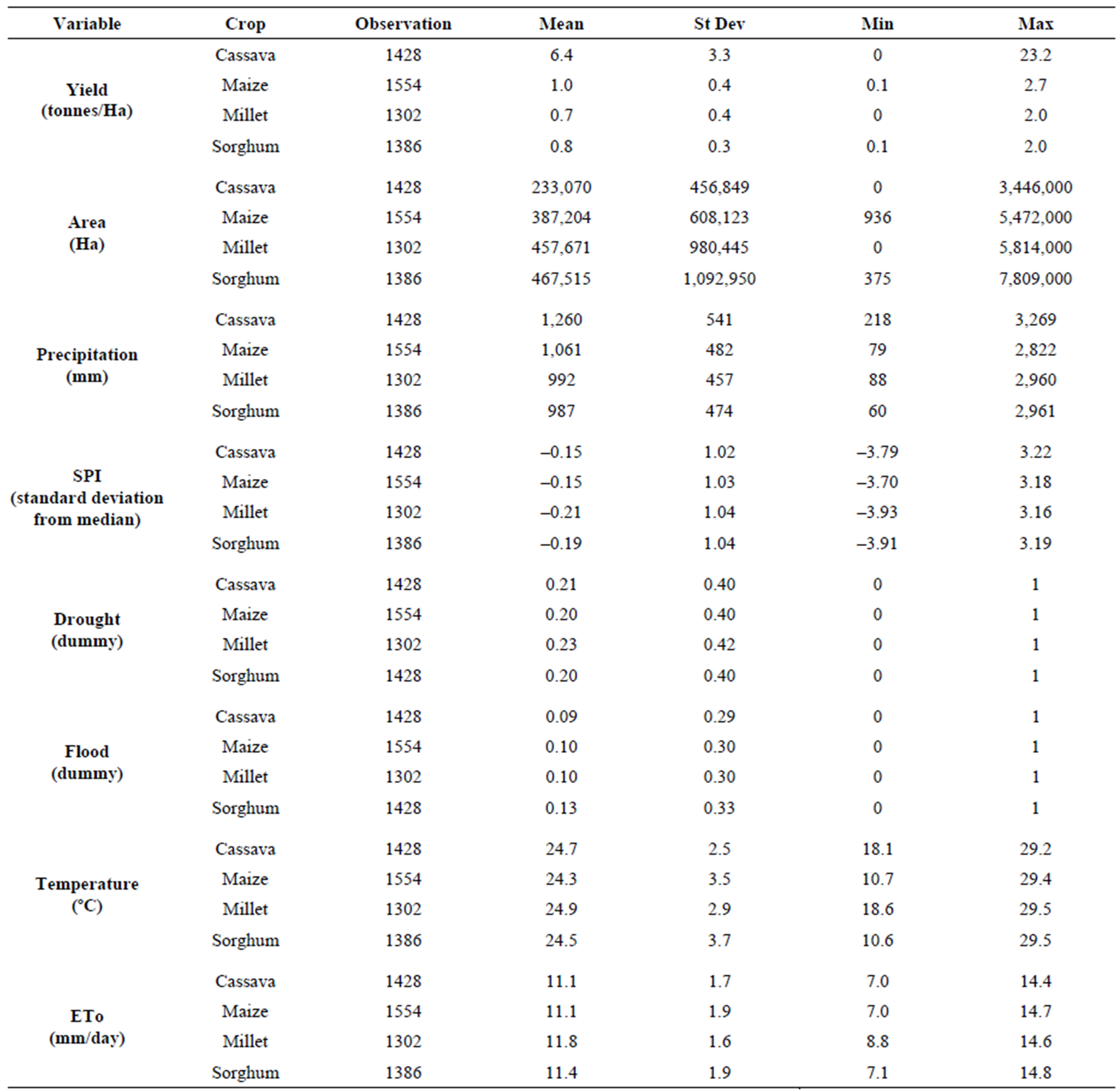
Table 1. SSA Summary statistics (1961-2002).
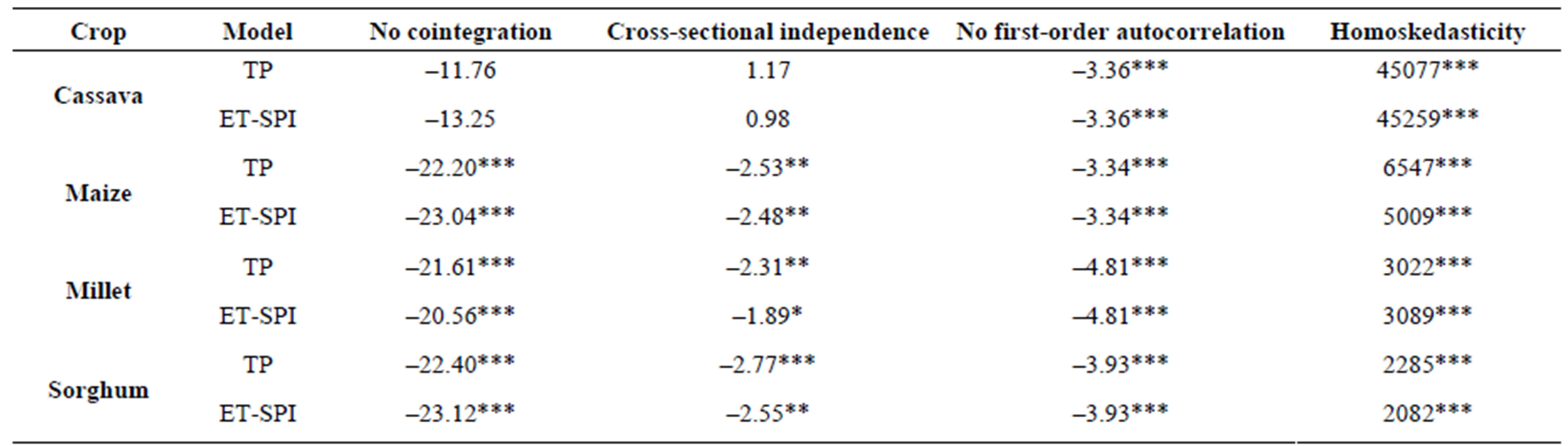
Table 2. Diagnostic tests statistics for final specifications.
fixed effect (FE) estimator, or if FEs are not significant, a pooled ordinary least squares (OLS) estimator, both with Driscoll and Kraay standard errors (1998). Driscoll and Kraay standard errors are robust to first-order correlation and heteroskedasticity and cross-sectional dependence. For consistency, the same estimator is used for each specification.
Regression results for the T-P and ET-SPI models are presented in Table 3. Regressions for the CO2 model showed a significant (and positive) effect of CO2 concentrations millet only. Results for the CO2 model are therefore not reported.
The estimated coefficient for the error correction term, ECt–1, is highly significant in maize, millet and sorghum regressions, which supports the cointegration test results. Estimated ECt–1 terms are similar for maize and millet and indicate that around 39% of the disequilibrium is corrected each year. For sorghum, the ECt–1 terms are slightly higher in magnitude (–0.49), indicating faster adjustment to equilibrium.
An increase in harvested area has a negative and significant effect on cassava, maize and sorghum yields, indicating decreasing marginal land productivity. For these three crops, estimated coefficients are similar in both T-P and ET-SPI models but differ across crops reflecting different marginal land productivities. For instance, a 10% increase in area causes a 2% cassava yield decrease, a 1.1% maize yield decrease, and a 0.9% sorghum yield decrease.
Regarding weather variables, as noted above, insignificant interaction and quadratic weather terms were excluded. For cassava, temperature and precipitations coefficients are not significant in the T-P regression. Similarly, ETo and SPI are insignificant in the ET-SPI model. However, the ET-SPI model indicates that floods are detrimental to cassava yields. Drought variables were insignificant and therefore excluded from the final specification reported in Table 3. This finding is plausible as cassava is a relatively drought resistant plant but vulnerable to excessive water.
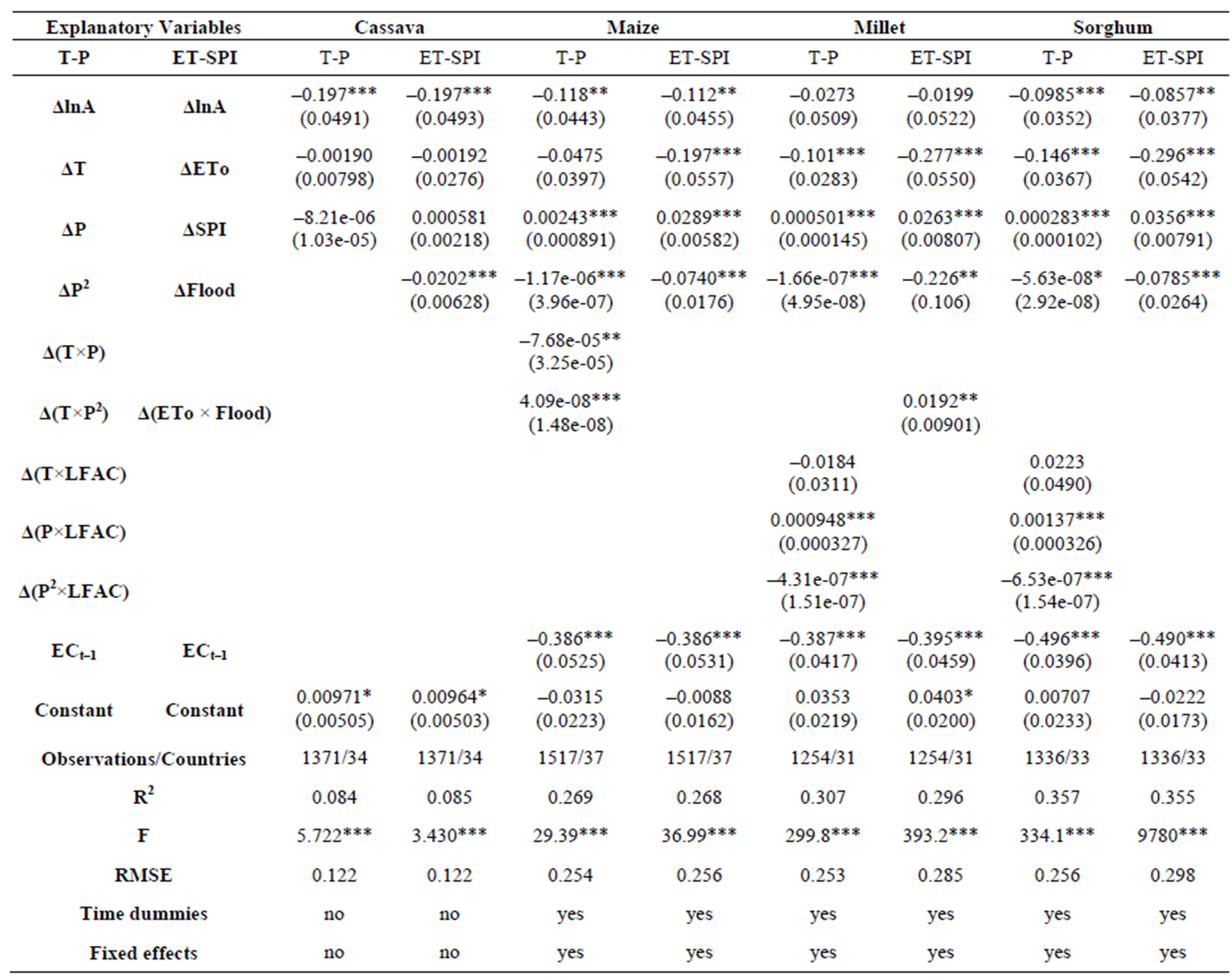
Table 3. T-P and ET-SPI regressions results: dependent variable ΔlnY.
Temperature and precipitation changes have the expected effects on maize yields. The significant squared precipitation term indicates non-linear yield responses to changes in precipitation. Also, the temperature and precipitation interaction terms reveal that the effect of precipitation depends on temperature and vice versa. Predicted values for ΔlnY for given values of P and T, and 90% confidence intervals, are represented in Figure 1. The left-hand graph shows that when P is at its mean value (1057 mm), a 1˚C temperature increase decreases maize yields by 8.3%. The right-hand graph illustrate that there is a concave relationship between precipitation and yield. When T is at its mean value (24.3˚C), a 100 mm increase in precipitation leads to a 1.7% maize yield increase. However, as the change in precipitation increases, the marginal impact of precipitation decreases. For a 500 mm increase in precipitation, yields increase by 3.1%.
The ET-SPI regressions provide a simpler representation of weather effect on maize than the T-P model. The ETo parameter has a significant negative effect on maize yield changes, which is consistent with expectations as an increase evapotranspiration is related to higher solar radiation and temperature. The SPI coefficient is positive and significant which indicates that higher than normal precipitation is beneficial to maize yields. For instance, a one standard deviation change from median precipitation increases maize yields by 2.9%. Alternatively, floods have a significant negative effect on yield. For example, maize yields during flood spells are respectively 7.1%, lower than during normal conditions in SSA.
In the T-P model, temperature has a negative and significant effect on millet yields. Precipitation has a positive effect on millet productivity and the squared precipitation term indicates a concave relationship between precipitation and yield. However, precipitation effects differ across LFAC and non-LFAC countries. As illustrated in Figure 2, a 100 mm decrease in precipitation leads to a 1.9% yield decrease in non-LFAC countries and a 3.3% yield decrease in LFAC countries. A 100mm increase in precipitation causes yield increases of 1.6% and 2.1% in non-LFAC and LFAC countries respectively. These findings are consistent with the expectation that crop growth in non-LFAC countries is less affected by weather events than in LFAC countries.
The ET-SPI model indicates a negative and significant ETo effect on millet yield, and the impact of ETo depends on flood occurrences and vice versa. Everything else constant, when Flood is at its mean value (0.09), a 0.5 mm per day increase in ETo causes a 13.8% decrease in millet yields. Alternatively, holding ETo at its mean value (11.8 mm/day), millet yields decrease by 0.02% when a flood starts.
The T-P model indicates that temperature has a negative impact on sorghum yields and precipitation has a positive
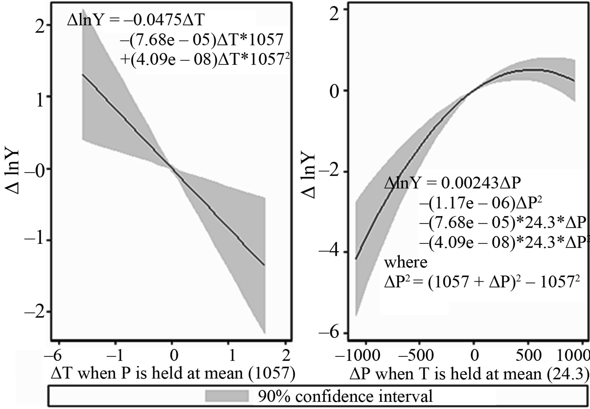
Figure 1. The effects of temperature and precipitation on maize yield.
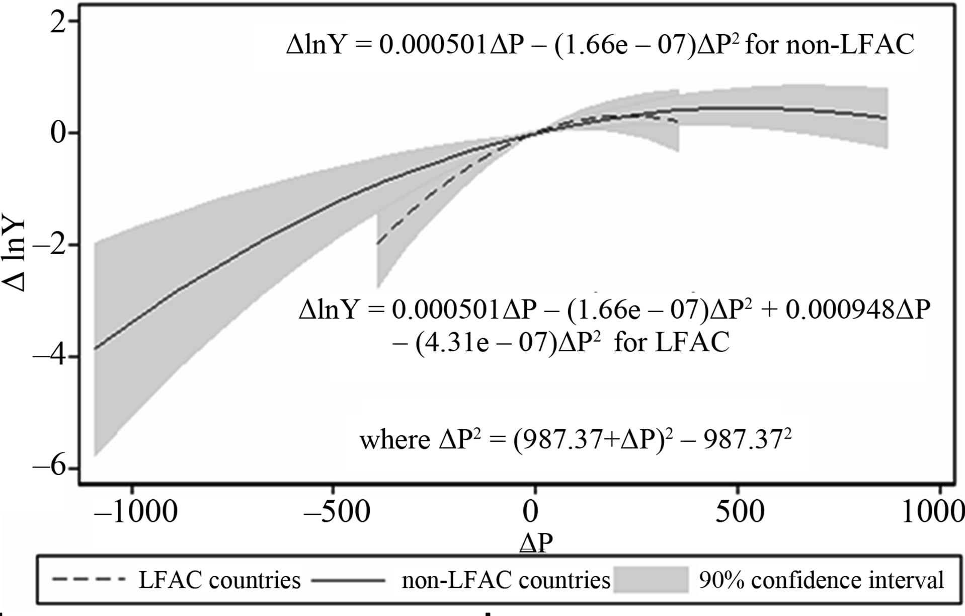
Figure 2. The effect of precipitation on millet yield.
non-linear effect on sorghum yields. Additionally, as for millet, precipitation has a larger effect on yields in LFAC countries than in non-LFAC countries. As displayed in Figure 3, a 100 mm increase in precipitation leads to a 1.7% increase in sorghum yields in non-LFAC countries and a 1.9% increase in LFAC countries. But the inclusion of the squared precipitation term implies a decreasing response at the margin. Therefore, a 200 mm change in precipitation leads to a sorghum yield increase of only 3.2% in non-LFAC countries and 2.4% in LFAC countries. The results illustrate that sorghum yields in LFAC countries are more vulnerable to precipitation changes than in non-LFAC countries.
Sorghum ET-SPI regressions results are similar to results for the T-P specification. ETo has a negative and significant effect on sorghum yields in SSA. A 1mm increase in ETo leads to a 29.6% increase in sorghum yields. These effects appear very important but represent extreme events. For an ETo increase of 0.006 mm (the average change in the sample), sorghum yields are expected to increase by only 0.18%. The SPI variable has a significant effect on sorghum yields. For example, a one standard deviation increase from median precipitation

Figure 3. The effect of precipitation on sorghum yield.
leads to a 3.6% sorghum yield increase. The effect of excessive precipitation, represented by flood dummies, is detrimental to sorghum yields. Specifically, sorghum yields during flood spells are 7.5% lower than during non-flood periods. These differences in predicted sorghum yields between flood and non-flood spell periods are similar to those estimated for maize.
5. Climate Change Predictions
Future climate changes are predicted using five atmosphere-ocean general circulation models (AOGCMs): CSIRO2 [69], HadCM3 [70], CGCM2 [71], ECHAM4 [72] and PCM [73]. Four alternative future GHG emissions scenarios serve as inputs into the AOGCMs. The four storylines that support the Special Report on Emissions Scenarios (SRES) scenarios (A1FI, A2, B1 and B2) are sourced from IPCC [74]. The storylines differ with respect to assumptions regarding population growth, economic and social development, energy and technology, and agriculture and land-use emissions. Based on the five AOGCMs and the four scenarios presented above, 20 future climate change scenarios are produced. Data for the four climate scenarios under the five AOGCMs are extracted from the TYN SC 2.0 dataset. The TYN SC 2.0 dataset provides global data at the 0.5 × 0.5 degree resolution from 2003 to 2100.
Over the 21st century, temperature is predicted to increase under all scenarios. Averaged across models, the largest temperature increases are predicted under the A1FI scenario, which predicts the largest increase in GHG emissions. Alternatively, the smallest temperature increase is predicted under the B1 scenario, which predicts the lowest level of CO2 concentration by 2100. Temperature increases also vary across AOGCMs. The ECHAM4 and HadCM3 models generally predict the highest temperatures, while the PCM model predicts the lowest temperatures. Evapotranspiration predictions for the 21st century are similar to those for temperature.
Precipitation predictions for the period 2003-2100 areon average, lowest under the A1FI and A2 scenarios and highest under the B2 scenario in all crop zones. Across AOGCMs, the lowest precipitation predictions over the 21st century are, on average, obtained from the CGCM2 model and the largest are obtained from the ECHAM4 model. Predicted SPI values follow similar patterns to precipitation values. The A1FI scenario produces the most frequent drought and flood occurrences, and the B1 scenario the fewest drought and flood occurrences. Compared to late-1900, droughts are generally expected to decrease, but increase in the CSIRO2 and HadCM3 models in late-2000. Flood occurrences are predicted to become less frequent under the CGCM2 model and more frequent under the ECHAM4 model.
6. Climate Change Impacts
In this study, the yield predictions for each crop are performed using the specification that best fits the data. The most widely used statistics used to assess predictive performance is the root mean squared error (RMSE) [75]. RMSE is calculated using the leave-one-out cross-validation (LOOCV) method described by Michaelsen [76].
As indicated in Table 3, The RMSE for the T-P and ET-SPI models are similar for cassava regressions. The ET-SPI model is preferred to predict cassava yields, as weather variables are insignificant in the T-P regression, while floods have a significant effect in the ET-SPI regression. For maize, the RMSE is slightly smaller for the T-P model than the ET-SPI model. However, the ET-SPI model is preferred to the T-P model as all weather variables in the ET-SPI are significant and the specification is simpler than the T-P. To predict millet yields, both the T-P and ET-SPI models produce similar estimates, so the choice is based on the RMSE, which indicates that the T-P model produces the best predictions. Regarding sorghum, the T-P model is preferred as it has a lower RMSE than the ET-SPI model.
To simplify presentation of climate change representations, average values for weather parameters are calculated over three 30-year periods. Average values over the period 1970 to 1999 represent the base period (late-1900), values over the period 2040 to 2059 represent mid-century forecasts (mid-2000) and values over the period 2070 to 2099 represent end of century predictions (late-2000).
Predicted cassava yields are very similar under all AOGCMs and scenarios. On average, cassava yields are expected to increase from 6.6 tonnes per Ha in late-1900 to 14.9 tonnes per Ha in late-2000 under all climate change scenarios. Maize yield predictions are generally the lowest under the B2 scenario, and highest under the A1FI scenario. By late-2000, maize yields are predicted to range from 2.6 tonnes/Ha under the scenario predicting the highest rate of evapotranspiration (HadCM3-A1FI), to 3.4 tonnes/Ha under the scenario predicting the lowest rate of evapotranspiration (PCM-B2). Compared to yields of 1 tonne/Ha in late-1980, these changes represent increases of 160% to 240% respectively. These predicted yield increases appear large, but are nevertheless below the maximum attainable yield of 5.1 tonne/Ha [77]. Regarding millet, compared to an average of 0.7 tonnes/Ha in late-1900, yield changes are predicted to range by between –28.6% under the HadCM3-A1FI, CGCM2-A1FI and ECHAM4-A1FI scenarios (0.5 tonnes/Ha), to 14.3% under the PCM-B1 (0.8 tonnes/Ha) by late-2000. Sorghum yields are predicted to increase under all scenarios and AOGCMs by mid-2000 but some decreases are predicted by late-2000 under the A1FI scenario. Specifically, predicted sorghum yields range from 0.8 tonnes/Ha under the HadCM3-A1FI, CGCM2-A1FI and ECHAM4- A1FI scenarios to 1.4 tonnes/Ha under the PCM-B1 scenario (i.e. changes of 0% to +75%, respectively, compared to late-1900).
The range of predicted climate change induced impacts in late-2000 on mean yield compared to the reference scenario of no climate change are presented in Figure 4. In this diagram, the boxes represent, for each crop and each scenario, the range of predictions across all AOGCMs between the 25th and 75th percentile. The lines inside the boxes represent the median predictions. The whiskers represent upper and lower adjacent values, unless a prediction is classified as an outsider, which is represented by hollow circles.
As can be seen in Figure 4, predictions for all crops are most widely spread under the A1FI scenario. The A1FI scenario predicts the largest temperature increasesthe largest precipitation changes (which increase or decrease depending on the AOGCM), and the largest changes in droughts and floods. Alternatively, the smallest variations in climate change impacts are predicted under the B1 scenario, which predicts the smallest increase in temperature and smallest changes in precipitation, droughts and floods. The box plot also shows that predicted yield impacts are negative for most crops. However, as in-sample predictions for cassava did not fit the data as well as predictions for other crops, predicted changes for this crop should be interpreted with caution.
Maize yield decreases relative to the reference scenario are predicted under nearly all scenarios by late-2000, and reach 18.8% under the HadCM3-A1FI scenario. However, a gain of up to 6.3% is predicted under the B2 scenario. Millet yields are predicted to decrease in all climate scenarios compared to the reference scenario. Yield decreases range from 37.5% under the HadCM3-A1FI, CGCM2-A1FI and ECHAM4-A1FI scenarios to 12.5% under other scenarios. Compared to the reference scenario, climate change causes sorghum yields decreases ranging from 46.7% under the HadCM3-A1FI, CGCM2- A1FI and ECHAM4-A1FI scenarios, to 6.7% under the PCM-B1 scenario by late-2000.
7. Conclusions
Analyses of the four most commonly harvested crops in SSA reveal, in general, a significant impact of weather on yields. Regression analyses using temperature and precipitation provided significant and sensible estimates.
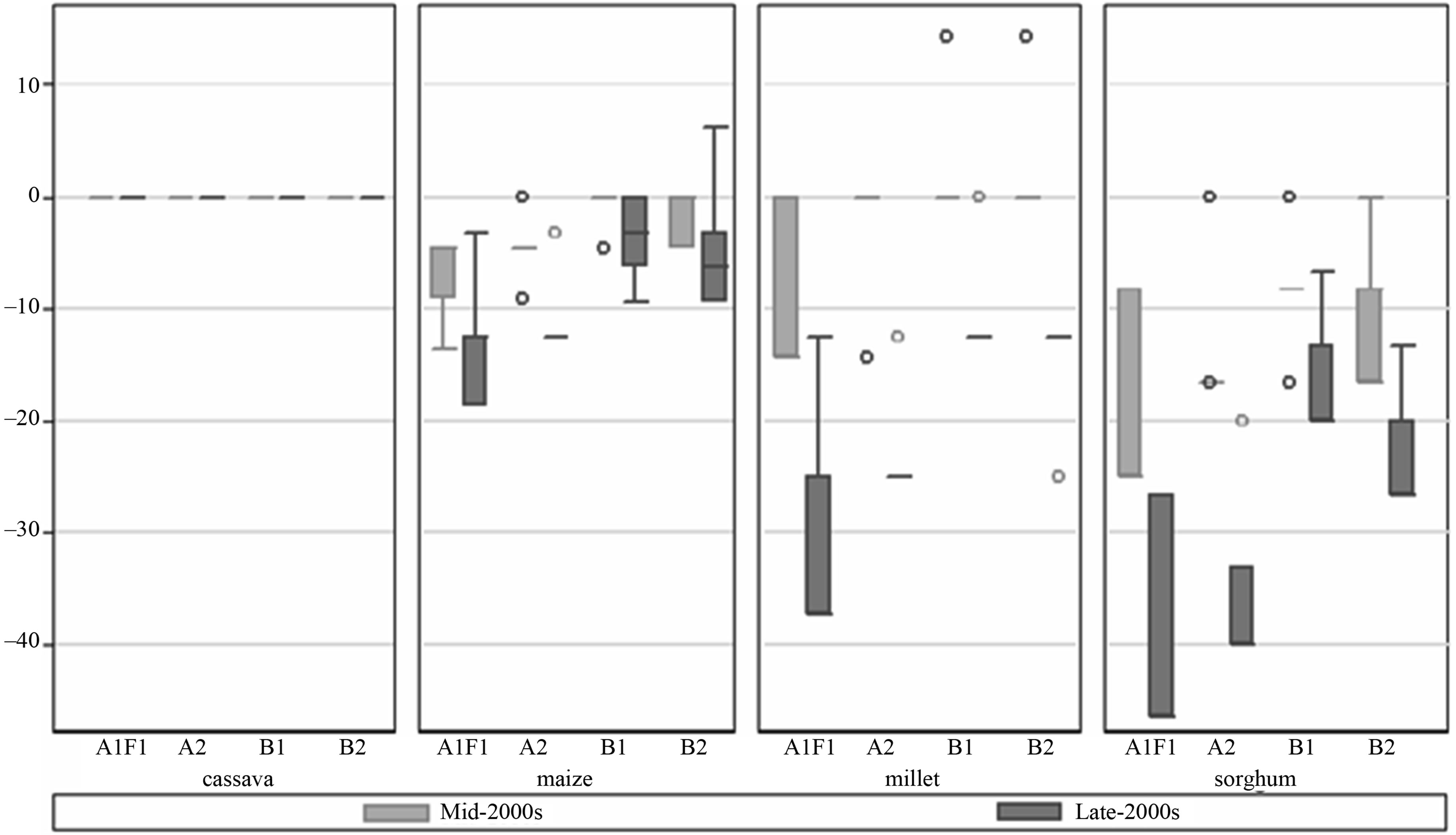
Figure 4. Predicted impact of climate change, compared to the reference scenario.
A second set of regressions using more refined weather parameters provided generally similar findings but with an explicit treatment of extreme precipitation events. The analysis also revealed that the impact of precipitation on crop yields depends on national agricultural conditions. Precipitation changes were found to have a larger impact on millet and sorghum yields in LFAC countries than non-LFAC countries.
These estimates were used to estimate the impact of future climate change. These calculations showed that, on average, crop yield are expected to increase in the 21st century compared to late-1900. However, compared to a scenario of no climate change, climate change is predicted to decrease yields for all crops, expect cassava. Comparing predictions across scenarios showed that climate impacts are smallest under the B1 scenario, which assumes reduced GHG emissions via, among other things, the introduction of clean and resource-efficient technologies and focusing on global solutions to economic, social and environmental sustainability.
When drawing conclusions from the results, it should be noted that predictions of the impact of climate change are beset by uncertainty. First, econometric based projections induce parameter and modeling uncertainty. The consideration of a confidence interval provides a measure of the uncertainty stemming from the econometric estimation. However, econometric estimates assume that the estimates based on past events will continue in the future. Second, the study produces predictions based on climate change predictions limited to the crop zones defined by Leff et al. [68], which are representative of the early 1990s. Therefore, the analysis fails to take into account the adaptation of farmers via spatial migration of crop zones. Third, there is uncertainty in climate change predictions stemming from climate modeling and future scenarios of GHG emissions due to incomplete or unknowable knowledge (New and Hulme, 2000). This study attempted to address this shortcoming by considering an ensemble of AOGCMs and scenarios, so as to provide a comprehensive range of potential impacts.
8. Acknowledgements
I am grateful for financing from the University of Otago and the MIT Joint Program on the Science and Policy of Global Change. I would also like to thank Niven Winchester, Paul Thorsnes and David Fielding for their help.
REFERENCES
- UNDP, “Climate Change and the Millennium Development Goals,” 1998. http://www.undp.org/climatechange/cc_mdgs.shtml
- O. Badiane and C. L. Delgado, “A 2020 Vision for Food, Agriculture, and the Environment in Sub-Saharan Africa,” International Food Policy Research Institute, Washington. DC, 1995.
- J. Rockström, C. Folke, L. Gordon, N. Hatibu, G. Jewitt, F. Penning De Vries, F. Rwehumbiza, H. Sally, H. Savenije and R. Schulze, “A Watershed Approach to Upgrade Rainfed Agriculture in Water Scarce Regions through Water System Innovations: An Integrated Research Initiative on Water for Food and Rural Livelihoods in Balance with Ecosystem Functions,” Physics and Chemistry of the Earth, Vol. 29, 2004, pp. 1109-1118. doi:10.1016/j.pce.2004.09.0016
- C. Rosenzweig and M. L. Parry, “Potential Impacts of Climate Change on World Food Supply,” Nature, Vol. 367, No. 13, 1994, pp. 133-138.
- S. Barrios, B. Ouattara and E. Strobl, “The Impact of Climatic Change on Agricultural Production: Is It Different for Africa?” Food Policy, Vol. 33, No. 4, 2008, pp. 287- 298. doi:10.1016/j.foodpol.2008.01.003
- A. Ben Mohamed, N. Van Duivenbooden and S. Abdoussallam, “Impact of Climate Change on Agricultural Production in the Sahel-Part 1: Methodological Approach and Case Study for Groundnut and Cowpea in Niger,” Climatic Change, Vol. 54, No. 3, 2002, pp. 327-348. doi:10.1023/A:1016189605188
- N. Van Duivenbooden, S. Abdoussallam and A. Ben Mohamed, “Impact of Climate Change on Agricultural Production in the Sahel-Part 2: Methodological Approach and Case Study for Millet in Niger,” Climatic Change, Vol. 54, No. 3, 2002, pp. 349-368. doi:10.1023/A:1016188522934
- W. Schlenker and D. B. Lobell, “Robust Negative Impacts of Climate Change on African Agriculture,” Environmental Research Letters, Vol. 5, No. 1, 2010, pp. 1-8. doi:10.1088/1748-9326/5/1/014010
- B. Oury, “Allowing for Weather in Crop Production Model Building,” American Journal of Agricultural Economics, Vol. 47, No. 2, 1965, pp. 270-283. doi:10.2307/1236574
- M. Upton, “African Farm Management,” Cambridge University Press, Cambridge, 1987.
- IAC, “Realizing the Promise and Potential of African Agriculture,” Internet Academy Council, 2004.
- FAO/AGL, “Terrastat Database,” 2009. http://www.fao.org/ag/agl/agll/terrastat/
- FAO, “The State of Food and Agriculture: Lessons from the Past 50 Years,” Food and Agricultural Organization of the United Nations, Rome, 2000.
- M. G. Wolman and F. G. A. Fournier, “Agricultural Practices Leading to Land Transformation: Introduction,” In: M. G. Wolman and F. G. A. Fournier, Eds., Land Transformation in Agriculture, John Wiley & Sons, Chichester, 1987, p. 531.
- F. Zaal, T. Dietz, J. Brons, K. Van Der Geest and E. Ofori-Sarpong, “Sahelian Livelihoods on the Rebound: A Critical Analysis of Rainfall, Drought Index and Yields in Sahelian Agriculture,” The Impact of Climate Change on Drylands, Vol. 39, 2004, pp. 61-77. doi:10.1007/1-4020-2158-5_7
- H. Larsson, “Relationships between Rainfall and Sorghum, Millet and Sesame in the Kassala Province, Eastern Sudan,” Journal of Arid Environments, Vol. 32, No. 2, 1996, pp. 211-223. doi:10.1006/jare.1996.0018
- A. M. Fermont, P. J. A. Van Asten, P. Tittonell, M. T. Van Wijk and K. E. Giller, “Closing the Cassava Yield Gap: An Analysis from Smallholder Farms in East Africa,” Field Crops Research, Vol. 112, No. 1, 2009, pp. 24-36. doi:10.1016/j.fcr.2009.01.009
- P. D. Jones and M. Hulme, “Calculating Regional Climatic Time Series for Temperature and Precipitation: Methods and Illustrations,” International Journal of Climatology, Vol. 16, No. 4, 1996, pp. 361-377. doi:10.1002/(SICI)1097-0088(199604)16:4<361::AID-JOC53>3.0.CO;2-F
- T. B. McKee, N. J. Doesken and J. Kleist, “The Relationship of Drought Frequency and Duration to Time Scales,” 8th Conference on Applied Climatology, California, 17-22 January 1993, pp. 179-184.
- C. F. Yamoah, G. E. Varvel, C. A. Francis and W. J. Waltman, “Weather and Management Impact on Crop Yield Variability in Rotations,” Journal of Production Agriculture, Vol. 11, No. 2, 1998, pp. 219-225.
- C. F. Yamoah, G. E. Varvel and J. Adu-Gyamfi, “Preplant Moisture and Fertility Conditions as Indicators of High and Stable Yields in Rainfed Cropping Systems,” Food Security in Nutrient Stressed Environments: Exploiting Plants’ Genetic Capabilities—Summary and Recommendations of an International Workshop, Patancheru, 27-30 September 1999, pp. 114-115.
- B. Narasimhan and R. Srinivasan, “Development and Evaluation of Soil Moisture Deficit Index (SMDI) and Evapotranspiration Deficit Index (ETDI) for Agricultural Drought Monitoring,” Agricultural and Forest Meteorology, Vol. 133, No. 1-4, 2005, pp. 69-88. doi:10.1016/j.agrformet.2005.07.012
- R. A. Seiler, M. Hayes and L. Bressan, “Using the Standardized Precipitation Index for Flood Risk Monitoring,” International Journal of Climatology, Vol. 22, No. 11, 2002, pp. 1365-1376. doi:10.1002/joc.779
- S. Quirogua and A. Iglesias, “Methods for Drought Risk Analysis in Agriculture,” Options Méditerranéennes, Vol. 58, 2007, pp. 103-113.
- A. Iglesias and S. Quirogua, "Measuring the risk of climate variability to cereal production at five sites in Spain", Climate Research, Vol. 34, 2007, pp. 47-57.
- E. Strobl, R.O. Strobl, "The distributional impact of large dams: Evidence from cropland productivity in Africa", Journal of Development Economics, Vol. 96, No. 2, 2010, pp. 1-19.
- P. A. O. Odjugo, “The Impact of Tillage Systems on Soil Microclimate, Growth and Yield of Cassava (Manihot utilisima) in Midwestern Nigeria,” African Journal of Agricultural Research, Vol. 3, No. 3, 2008, pp. 225-233.
- D. B. Lobell and C. B. Field, “Global Scale Climate-Crop Yield Relationships and the Impacts of Recent Warming,” Environmental Research Letters, Vol. 2, No. 1, 2007, pp. 1-7. doi:10.1088/1748-9326/2/1/014002
- C.-C. Chen, B. A. McCarl and D. Schimmelpfennig, “Yield Variability as Influenced by Climate: A Statistical Investigation,” Climatic Change, Vol. 66, No. 2, 2000, pp. 239- 261. doi:10.1023/B:CLIM.0000043159.33816.e5
- C. J. Kucharik and S. P. Serbin, “Impacts of Recent Climate Change on Wisconsin Corn and Soybean Yield Trends,” Environmental Research Letters, Vol. 3, No. 3, 2008, pp. 1-10. doi:10.1088/1748-9326/3/3/034003
- N. Maman, D. J. Lyon, S. Mason, T. D. Galusha and R. Higgins, “Pearl Millet and Grain Sorghum Yield Response to Water Supply in Nebraska,” Agronomy Journal, Vol. 95, No. 16, 2003, pp. 1618-1624.
- G. Abbas, A. Hussain, A. Ahmad and S. A. Wajid, “Water Use Efficiency of Maize as Affected by Irrigation Schedules and Nitrogen Rates,” Journal of Agriculture & Social Sciences, Vol. 1, No. 4, 2005, pp. 339-342.
- R. K. Pandey, J. W. Maranville and A. Admou, “Deficit Irrigation and Nitrogen Effects on Maize in a Sahelian Environment: I. Grain Yield and Yield Components,” Agricultural Water Management, Vol. 46, No. 1, 2000, pp. 1-13. doi:10.1016/S0378-3774(00)00073-1
- G. H. Hargreaves and Z. A. Samani, “Reference Crop Evapotranspiration from Temperature,” Applied Engineering in Agriculture, Vol. 1, No. 2, 1985, pp. 96-99.
- R. G. Allen, L. S. Pereira, D. Raes and M. Smith, “Crop Evapotranspiration—Guidelines for Computing Crop Water Requirements,” FAO Irrigation and Drainage Paper, FAO, Rome, 1998.
- M. Morris, V. A. Kelly, R. J. Kopicki and D. Byerlee, “Fertilizer Use in African Agriculture: Lessons Learned and Good Practice Guidelines,” In: Directions in Development—Agriculture and Rural Development, World Bank, Washington DC, 2007. doi:10.1596/978-0-8213-6880-0
- FAO, “Fertilizer Requirements in 2015 and 2030 Revisited,” FAO, Rome, 2004.
- J.-M. Faurès and G. Santini, “Water and the Rural Poor— Interventions for Improving Livelihoods in Sub-Saharan Africa,” FAO, Land and Water Division, Rome, 2008.
- FAO, “Seed Policy and Programmes for Sub-Saharan Africa: Proceedings of the Regional Technical Meeting on Seed Policy and Programmes for Sub-Saharan Africa,” Food and Agriculture Organization of the United Nations, Rome, 1998.
- T. Teklu, J. V. Braum and E. Zaki, “Drought and Famine Relationships in Sudan: Policy Implication,” International Food Policy Research Institute (IFPRI), 1991.
- C. F. Yamoah, D. T. Walters, C. A. Shapiro, C. A. Francis and M. J. Hayes, “Standardized Precipitation Index and Nitrogen Rate Effects on Crop Yields and Risk Distribution in Maize,” Agriculture Ecosystems & Environment, Vol. 80, No. 1-2, 2000, pp. 113-120. doi:10.1016/S0167-8809(00)00140-7
- R. W. Malone, D. W. Meek, J. L. Hatfield, M. E. Mann, R. J. Jaquis and L. Ma, “Quasi-Biennial Corn Yield Cycles in Iowa,” Agricultural and Forest Meteorology, Vol. 149, No. 6-7, 2009, pp. 1087-1094. doi:10.1016/j.agrformet.2009.01.009
- S. Shaik and G. A. Helmers, “Intertemporal and Interspatial Variability of Climate Change on Dryland Winter Wheat Yield Trends,” Agricultural Economics, University of Nebraska-Lincoln, Lincoln, 2000.
- P. Collier and African Studies Association Meeting, “Africa and the Study of Economics,” In: R. H. Bates, V. Y. Mudimbe and J. F. O’Barr, Eds., Africa and the Disciplines: The Contribution of Research in Africa to the Social Sciences and Humanities, University of Chicago Press, Chicago, 1993.
- J. A. Dixon, A. Gulliver and D. P. Gibbon, “Farming Systems and Poverty—Improving Farmers’ Livelihoods in a Changing World,” Food and Agriculture Organization of the United Nations and World Bank, 2001.
- X. Diao, P. Hazell, D. Resnick and J. Thurlow, “The Role of Agriculture in Development: Implications for Sub-Saharan Africa,” International Food Policy Research Institute (IFPRI), 2006.
- D. G. Kleinbaum, L. L. Kupper, A. Nizam and K. E. Muller, “Applied Regression Analysis and Other Multivariable Methods,” 4th Edition, Duxbury Press, Duxbury, 2008.
- Y. Ganzach, “Misleading Interaction and Curvilinear Terms,” Psychological Methods, Vol. 2, No. 3, 1997, pp. 235- 247. doi:10.1037/1082-989X.2.3.235
- K. Hadri, “Testing for Stationarity in Heterogeneous Panel Data,” The Econometrics Journal, Vol. 3, No. 2, 2000, pp. 148-161. doi:10.1111/1368-423X.00043
- A. Levin, C.-F. Lin and C.-S. J. Chu, “Unit Root Tests in Panel Data: Asymptotic and Finite Sample Properties,” Journal of Econometrics, Vol. 108, No. 1, 2002, pp. 1-24. doi:10.1016/S0304-4076(01)00098-7
- K. S. Im, M. H. Pesaran and Y. Shin, “Testing for Unit Roots in Heterogeneous Panels,” Journal of Econometrics, Vol. 115, No. 1, 2003, pp. 53-74. doi:10.1016/S0304-4076(03)00092-7
- G. S. Maddala and S. Wu, “A Comparative Study of Unit Root Tests With Panel Data and a New Simple Test,” Oxford Bulletin of Economics and Statistics, Vol. 61, No. S1, 1999, pp. 631-652. doi:10.1111/1468-0084.0610s1631
- G. Elliott, T. J. Rothenberg and J. H. Stock, “Efficient Tests for an Autoregressive Unit Root,” Journal of Econometrics, Vol. 64, No. 4, 1996, pp. 813-836.
- D. Kwiatkowski, P. C. B. Phillips, P. Schmidt and Y. Shin, “Testing the Null Hypothesis of Stationarity against the Alternative of Unit Root,” Journal of Econometrics, Vol. 54, No. 1-3, 1992, pp. 159-178.
- G. S. Maddala and I.-M. Kim, “Unit Roots, Cointegration, and Structural Change,” Cambridge University Press, Cambridge, 1998.
- G. W. Schwert, “Tests for Unit Roots: A Monte Carlo Investigation,” Journal of Business and Economic Statistics, Vol. 7, 1989, pp. 147-160.
- P. Pedroni, “Panel Cointegration: Asymptotic and Finite Sample Properties of Pooled Time Series Tests with an Application to the PPP Hypothesis,” Econometric Theory, Vol. 20, No. 3, 2004, pp. 597-625. doi:10.1017/S0266466604203037
- P. Pedroni, “On the Role of Cross-Sectional Dependency in Panel Unit Root and Panel Cointegration Exchange Rate Studies,” Working Paper, Department of Economics, Indiana University, 1997.
- P. Pedroni, “Critical Values for Cointegration Tests in Heterogeneous Panels with Multiple Regressors,” Oxford Bulletin of Economics and Statistics, Vol. 61, No. S1, 1999, pp. 653-670. doi:10.1111/1468-0084.0610s1653
- S. McCoskey and C. Kao, “A Residual-Based Test of the Null of Cointegration in Panel Data,” Econometric Reviews, Vol. 17, No. 1, 1998, pp. 57-84. doi:10.1080/07474939808800403
- C. Kao, “Spurious Regression and Residual-Based Tests for Cointegration in Panel Data,” Journal of Econometrics, Vol. 90, 1999, pp. 1-44.
- J. Westerlund, “Testing for Error Correction in Panel Data,” Oxford Bulletin of Economics and Statistics, Vol. 69, No. 6, 2007, pp. 709-748. doi:10.1111/j.1468-0084.2007.00477.x
- W. H. Greene, “Econometric Analysis,” 4th Edition, Prentice Hall, Upper Saddle River, 2000.
- M. H. Pesaran, “General Diagnostic Tests for Cross Section Dependence in Panels,” Cambridge Working Papers in Economics, University of Cambridge, Cambridge, 2004.
- M. Arellano and S. Bond, “Some Tests of Specification for Panel Data: Monte Carlo Evidence and an Application to Employment Equations,” The Review of Economic Studies, Vol. 58, No. 2, 1991, pp. 277-297. doi:10.2307/2297968
- FAOSTAT, “FAO Statistical Databases,” 2007. http://faostat.fao.org
- T. D. Mitchell and P. D. Jones, “An Improved Method of Constructing a Database of Monthly Climate Observations and Associated High-Resolution Grids,” International Journal of Climatology, Vol. 25, No. 6, 2005, pp. 693-712. doi:10.1002/joc.1181
- B. Leff, N. Ramankutty and J. Foley, “Geographic Distribution of Major Crops across the World,” Global Biogeochemical Cycles, Vol. 18, 2004. doi:10.1029/2003GB002108
- H. B. Gordon and S. P. O’Farrell, “Transient Climate Change in the CSIRO Coupled Model with Dynamic Sea ice,” Monthly Weather Review, Vol. 125, No. 5, 1997, 875-907. doi:10.1175/1520-0493(1997)125<0875:TCCITC>2.0.CO;2
- C. Gordon, C. Cooper, C. A. Senior, H. Banks, J. M. Gregory, T. C. Johns, J. F. B. Mitchell and R. A. Wood, “The Simulation of SST, Sea Ice Extents and Ocean Heat Transports in a Version of the Hadley Centre coupled Model without Flux Adjustments,” Climate Dynamics, Vol. 16, No. 2-3, 2000, pp. 147-168. doi:10.1007/s003820050010
- G. M. Flato and G. J. Boer, “Warming Asymmetry in Climate Change Simulations,” Geophysical Research Letters, Vol. 28, No. 1, 2001, pp. 195-198.
- E. Roeckner, J. M. Oberhuber, A. Bacher, M. Christoph and I. Kirchner, “ENSO Variability and Atmospheric Response in a Global Coupled Atmosphere-Ocean GCM,” Climate Dynamics, Vol. 12, No. 11, 1996, pp. 737-754. doi:10.1007/s003820050140
- W. M. Washington, J. W. Weatherly, G. A. Meehl, A. J. Semtner Jr., T. W. Bettge, A. P. Craig, W. G. Strand Jr., J. Arblaster, V. B. Wayland, R. James and Y. Zhang, “Parallel Climate Model (PCM) Control and Transient Simulations,” Climate Dynamics, Vol. 16, No. 10-11, 2000, pp. 755-774. doi:10.1007/s003820000079
- IPCC, “Special Report on Emissions Scenarios,” Cambridge University Press, Cambridge, 2000.
- P. E. Kennedy, “A guide to Econometrics,” 5th Edition, The MIT Press, Cambridge, 2003.
- J. Michaelsen, “Cross-Validation in Statistical Climate Forecast Models,” Journal of Climate and Applied Meterorology, Vol. 26, 1987, pp. 1589-1600. doi:10.1175/1520-0450(1987)026<1589:CVISCF>2.0.CO;2
- G. Fischer, H. Van Velthuizen, M. Shah and F. Nachtergaele, “Global Agro-Ecological Assessment for Agriculture in the 21st Century: Methodology and Results,” International Institute for Applied Systems Analysis Laxenburg and Austria and Food and Agriculture Organization of the United Nations, Rome, 2002.
NOTES
1In this study, LFAC countries include Botswana, Burundi, Chad, Gabon, Madagascar, Mali, Mauritania, Namibia, Niger and Rwanda. Remaining countries are classified as non-LFAC countries.
2The KPSS stationarity test of Kwiatkowski et al. [54] is not used because of its low power [55].
3Although FAOSTAT provides data for all countries in SSA, several outlier countries are not considered in the analysis: Ethiopia and Eritrea, which were one nation (Ethiopia) prior to 1993; Djibouti, which produces very little agriculture; and South Africa, which employs farming practices similar to North American and European practices [37] and is very different from other SSAn countries. Additionally, millet agronomic data in Congo are not considered as data are only available from 2000.
4Some sorghum production is reported in Madagascar [66], but as crop location data do not report sorghum growing in this country, sorghum weather data are not available for this country.