International Journal of Modern Nonlinear Theory and Application
Vol.2 No.1(2013), Article ID:28671,6 pages DOI:10.4236/ijmnta.2013.21001
Stability Analysis of a Nonlinear Difference Equation
Department of Mathematics, Faculty of Education, Erciyes University, Kayseri, Turkey
Email: fbozkurt@erciyes.edu.tr
Received January 1, 2013; revised January 31, 2013; accepted February 9, 2013
Keywords: Difference Equations; Stability Analysis; Semi-Cycle Solutions; Boundedness
ABSTRACT
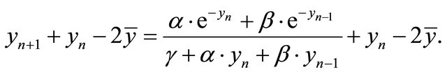
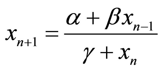
The local and global behavior of the positive solutions of the difference equation
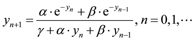
was investigated, where the parameters ,
,  and
and  and the initial conditions are arbitrary positive numbers. Furthermore, the characterization of the stability was studied with a basin that depends on the conditions of the coefficients. The analysis about the semi-cycle of positive solutions has end the study of this work.
1. Introduction
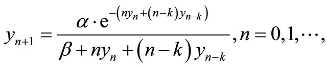
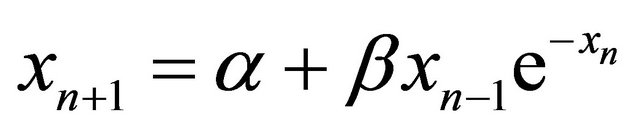
H. El-Metwally et al. [1] studied the global stability of the difference equation
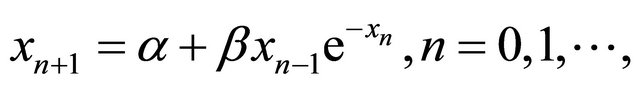 (1.1)
(1.1)
where the parameters  and
and  are positive numbers and the initial conditions are arbitrary non-negative real numbers. This equation may be viewed as a model in Mathematical Biology, where
  is the immigration rate and
  the population growth rate.
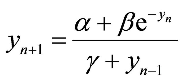
In [2] was investigated the globally asymptotically stability of the difference equation
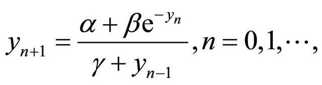 (1.2)
(1.2)
where the parameters ,
,  and
and  are positive numbers and the initial conditions are arbitrary non-negative numbers. In [3] the boundedness and the global asymptotic behavior of the difference equation
 (1.3)
(1.3)
was shown, where  and
and  are positive real numbers,
  and the initial conditions
 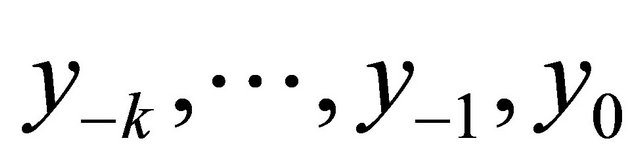 are arbitrary numbers. Similar studies can be shown in [4-7].
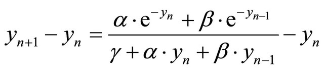
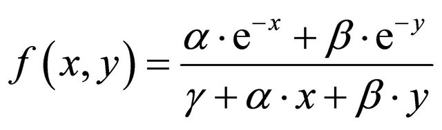
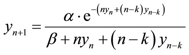
The aim in this paper is to study the local and global behavior of the positive solutions of the difference equation
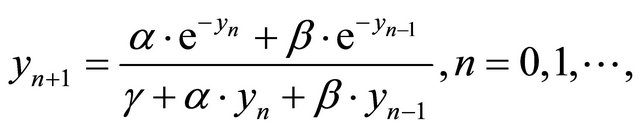 (1.4)
(1.4)
where the parameters ,
,  and
and  and the initial conditions are arbitrary positive numbers. In Section 2, the local asymptotic stability of the equilibrium point of Equation (1.4) was investigated by using the Linearized Stability Theorem. A suitable Lyapunov function for the analysis of the global asymptotic stability behavior was used, like the idea in [8,9]. Furthermore, the characterization of the stability was examined that depends on the conditions of the coefficients (see [10]). In Section 3, the semi-cycle of positive solutions was analyzed. All this results will be shown theoretical and by simulations at the end of the paper.
2. Local and Global Asymptotic Stability Analysis
In this section, we discuss the local and global asymptotic stability of the unique positive equilibrium point of Equation (1.4) by using the theorems in [4,8-10].
The equilibrium points of Equation (1.4) are the solutions of the equation
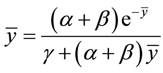 . (2.1)
Set
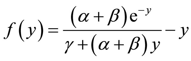 (2.2)
(2.2)
for  and
and  we obtain respectively,
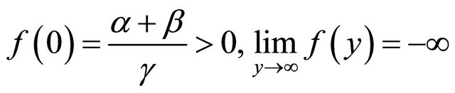 (2.3)
(2.3)
and
 . (2.4)
It follows that Equation (2.1) has exactly one solution . From this result Equation (1.4) has a unique equilibrium
 .
.
The linearized equation and the characteristic equation associated with Equation (1.4) about the equilibrium  is
is
 (2.5)
(2.5)
and
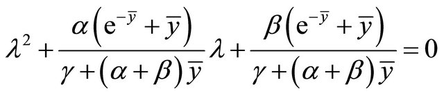 , (2.6)
respectively.
Theorem 2.1. The following statements are true.
1) Every solution of Equation (1.4) is bounded if .
.
2) The equilibrium point of Equation (1.4) is bounded if 
Proof.
1) Suppose that . Let
. Let  be a solution of Equation (1.4). We have
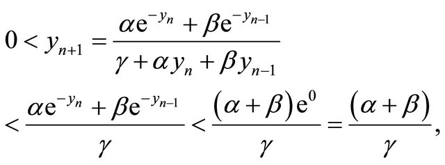
which gives that every positive solution of the Equation (1.4) is bounded. Thus 1) is true.
2) Assume that . Then
which implies that 2) is also true.
Theorem 2.2 Let . If
. If
 (2.7)
(2.7)
then the positive equilibrium point of Equation (1.4) is locally asymptotically stable.
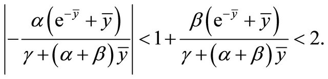
Proof. From the Linearized Stability Theorem, we can write
 . (2.8)
The inequality (2.8) can be shown under two cases;
1) 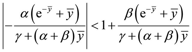
2) .
.
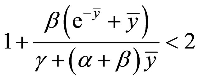
From 2), we get
 (2.9)
(2.9)
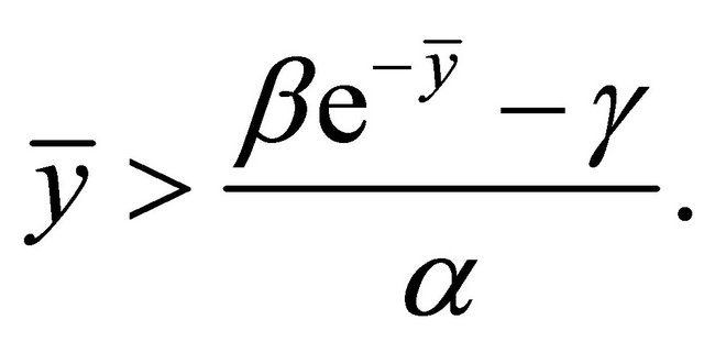
By 1), we will have
 (2.10)
which always holds and since , we can also obtain
 (2.11)
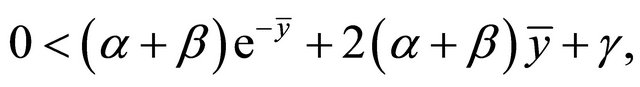
Considering both (2.9) and (2.11), if
then we have
 (2.12)
Rewriting (2.12), we get
 (2.13)
In view of (2.12) and (2.13), we obtain
 .
.
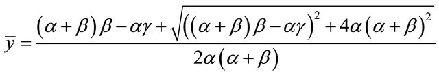
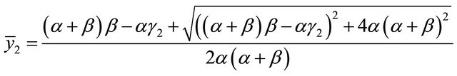
Theorem 2.3. Let the conditions in Theorem 2.2 hold and assume that  and
and  are the equilibrium points of Equation (1.4), which parameters have the conditions
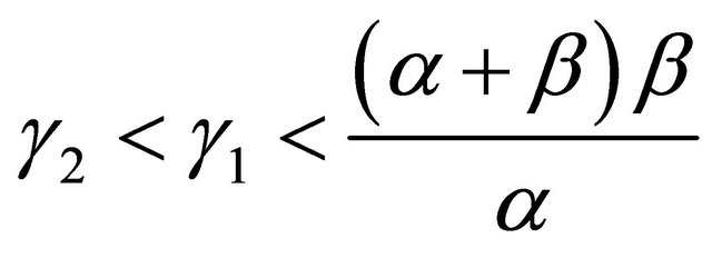 . If the parameter
  decreases, then the local stability of the positive equilibrium point
 (2.14)
decreases also.
Proof. By the Linearized Stability Theorem, we have
 (2.15)
Let
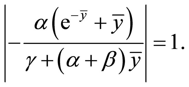 (2.16)
From (2.16), computations will give us
 (2.17)
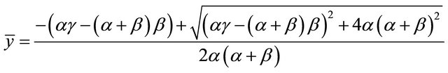
where we get the positive equilibrium point
 .
.
Let us write
 (2.18)
and
 , (2.19)
where 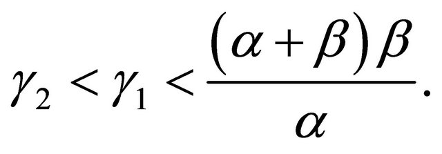
Considering both (2.18) and (2.19), we get
 (2.20)
On the other side, from (2.15), we will investigate
 (2.21)
From (2.21) assume that
 (2.22)
Considering the conditions in Theorem 2.2, if furthermore (2.22) holds, than the stability of  is weaker than
  By computing (2.22), we obtain
 (2.23)
This inequality can be also written in the form
 (2.24)
From (2.20) we get
 (2.25)
which always holds. This completes the proof.
Theorem 2.4. Suppose that  is a monoton decreasing solution of Equation (1.4) and assume that the conditions in Theorem 2.2 hold. If
 (2.26)
then the positive equilibrium point of Equation (1.4) is globally asymptotically stable.
Proof. We consider a Lyapunov function  defined by
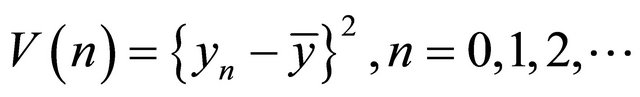 (2.27)
The change along the solutions of Equation (1.4) is
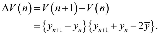 (2.28)
From (2.28) we can write
and
It can be compute that by using the hypothesis we have , which is the condition for the global asymptotic stability of the positive equilibrium point of Equation (1.4).
3. The Semi-Cycle and Oscillation
In this section, we consider the semi-cycle and oscillation of the positive solutions of Equation (1.4).
 (a)
(a)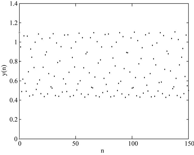 (b)
(b)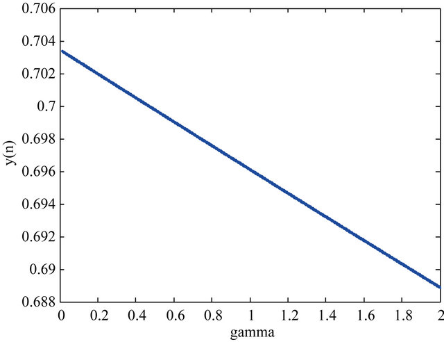 (c)
(c)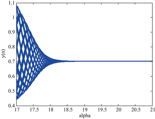 (d)
(d)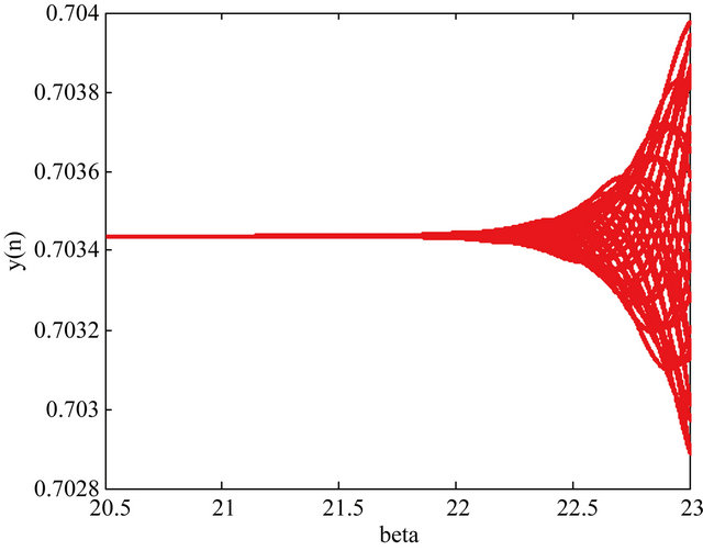 (e)
(e)
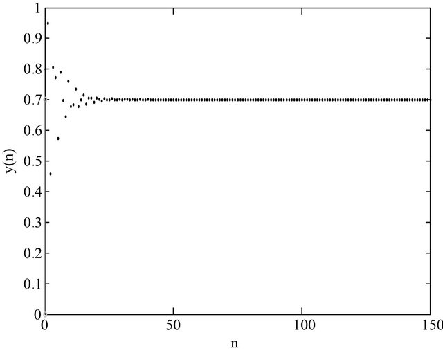
Figure 1. (a) Local stable behavior of Equation (1.4) for α = 30, β = 20, γ = 0.3, y(−1) = 0.8 and y(0) = 0.95; (b) Unstable behavior of Equation (1.4) for α = 20, β = 30, γ = 0.3, y(−1) = 0.8 and y(0) = 0.9; (c) Stability analysis for α = 30, β = 20, γ [0.01, 2], y(−1) = 0.8 and y(0) = 0.95; (d) Diagram of the solutions of Equation (1.4) for β = 30, α
 [17, 21], γ
 0.03, y(−1) = 0.8 and y(0) = 0.95; (e) Diagram of the solution of Equation (1.4) for α = 17.2, β
 [20.5, 23], γ
 0.003, y(−1) = 0.8 and y(0) = 0.95.
By [8], a positive semi-cycle of a solution 
of  consists of a “string” of terms
 , all greater than or equal to the equilibrium
 , with
  and
and  and such that either
  or
or  and
and  and either
  or
or  and
and .
.
A negative semi-cycle of a solution  of
of
 consists of a “string” of terms
 , all less than the equilibrium
 , with
  and
and  and such that either
  or
or  and
and  and either
  or
or  and
and .
.
Theorem B ([9]) Assume that  and that
  is decreasing in both arguments. Let
  be a positive equilibrium of
 . Then every oscillatory solution of the difference equation
 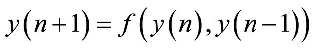 has semi-cycle of length at most two.
Theorem 3.2. Let 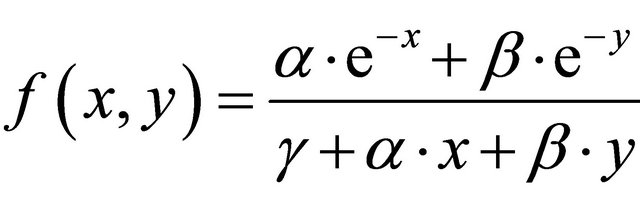 be a function such that
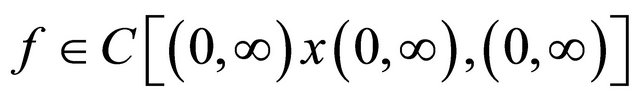 . Then every oscillatory solution of Equation (1.4) has semi-cycle of length at most two.
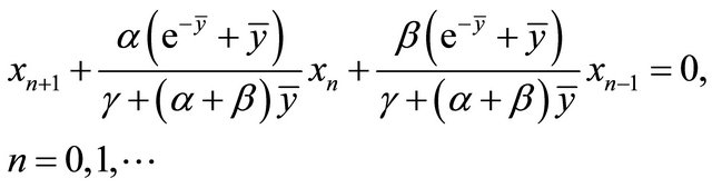
Proof. By the Theorem B, we can write Equation (1.4) such as
 . (3.1)
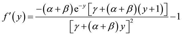
The first derivative of (3.1) with respect to x and y are
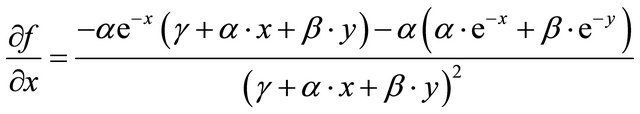 (3.2)
(3.2)
and
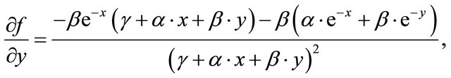 (3.3)
(3.3)
respectively. These derivatives are less than zero if
 (3.4)
(3.4)
and
 (3.5)
(3.5)
respectively. Since the parameters are positive and the variables x and y are in a positive interval, (3.4) and (3.5) will be always hold. This completes the proof.
Example 1 In this Example, Figure 1(a) show the local stability of Equation (1.4) for the parameters ,
,  ,
,  ,
,  and
and  by using the conditions in Theorem 2.2. The parameters
 ,
, 
 and the initial conditions
  and
and  are selected to show in Figure 1(b) the unstable behavior of the solutions of Equation (1.4). In Figure 1(c), we can show that by decreasing of the parameter
  the local stability get be weaker. At last, Figures 1(d) and (e) show the diagram of the solutions of Equation (1.4) for
 ,
,  ,
,  ,
,  and
and  and for
 ,
,  ,
,  ,
,  and
and , respectively. This give us the relation between the parameters
  and
and , which have an important role by the stability analysis of Equation (1.4), as shown in Theorem 2.2 and Theorem 2.4.
REFERENCES
- H. El-Metwally, E. A. Grove, G. Ladas, R. Levins and M. Radin, “On the Difference Equation
 ,” Nonlinear Analysis, Vol. 47, No. 7, 2001, pp. 4623-4634. doi:10.1016/S0362-546X(01)00575-2
 - I. Ozturk, F. Bozkurt and S. Ozen, “On the Difference Equation
 ,” Applied Mathematics and Computations, Vol. 181, No. 2, 2006, pp. 1387-1393. doi:10.1016/j.amc.2006.03.007
 - I. Ozturk, F. Bozkurt and S. Ozen, “Global Asymptotic Behavior of the Difference Equation
 ,” Applied Mathematic Letters, Vol. 22, No. 4, 2009, pp. 595-599. doi:10.1016/j.aml.2008.06.037
 - C. H. Gibbons, M. R. S. Kulenovic, G. Ladas and H. D. Voulov, “On the Trichotomy Character of
 ,” Journal of Difference Equations and Applications, Vol. 8, No. 1, 2002, pp. 75- 92. doi:10.1080/10236190211940
 - M. M. El-Afifi and A. M. Ahmed, “On the Difference Equation
 ,” Applied Mathematics and Computations, Vol. 144, No. 2-3, 2003, pp. 537-542. doi:10.1016/S0096-3003(02)00429-0
 - W. S. He and W. T. Li, “Attractivity ın a Nonlinear Delay Difference Equation,” Applied Mathematics E—Notes, Vol. 4, 2004, pp. 48-53.
- S. Ozen, I. Ozturk and F. Bozkurt, “On the Recursive Sequence
 ,” Applied Mathematics and Computation, Vol. 188, No. 1, 2007, pp. 180-188. doi:10.1016/j.amc.2006.09.106
 - K. Cunningham, et al., “On the Recursive Sequence
 ,” Nonlinear Analysis, Vol. 47, No. 7, 2001, pp. 4603-4614. doi:10.1016/S0362-546X(01)00573-9
 - C. Gibbons, M. R. S. Kulenovic and G. Ladas, “On the Recursive Sequence
 ,” Mathematical Sciences Research Hot-Line, Vol. 4, No. 2, 2000, pp. 1- 11.
 - C. Celik, H. Merdan, O. Duman and O. Akın, “Allee Effects on Population Dynamics with Delay,” Chaos, Solitons and Fractals, Vol. 37, No. 1, 2008, pp. 65-74.