Open Journal of Applied Sciences
Vol.3 No.4(2013), Article ID:34997,5 pages DOI:10.4236/ojapps.2013.34037
Forecasting Number of Students in University Department: Modeling Approach
1Department of Mathematics, Faculty of Applied Sciences, King Mongkut’s University of Technology North Bangkok Bangkok, Thailand
2Department of Mathematics, Faculty of Science, Silpakorn University, Bangkok, Thailand
Email: *nichaphatb@kmutnb.ac.th
Copyright © 2013 Nichaphat Patanarapeelert, Klot Patanarapeelert. This is an open access article distributed under the Creative Commons Attribution License, which permits unrestricted use, distribution, and reproduction in any medium, provided the original work is properly cited.
Received May 25, 2013; revised June 25, 2013; accepted July 2, 2013
Keywords: Student population; Regression analysis; Descriptive model; Explanatory model
ABSTRACT
In this study, the mathematical models of dynamics of student populations in the university departments are formulated. As a case study, we employ the data of registration section from Department of Mathematics, Faculty of Applied Science, King Mongkut’s University of Technology North Bangkok (KMUTNB), Thailand, from calendar year 2006 to 2010. Using regression analysis, descriptive model and explanatory model are derived. The descriptive model is linear with R2 = 0.8864. Using log-transformation, the explanatory model gives the nonlinear approximation with R2 = 0.8293. The model predicts that the number of students of Department of Mathematics, KMUTNB has a tendency to linearly increase with slope of 20 with 95% CI (6.8417, 33.1583). The application of the models in educational management is discussed.
1. Introduction
Full Time Equivalent Student (FTES) is a standard unit that is accepted to use for the purposes of measuring, comparing or assessing in educational management. Particular interest is calculation of the ratio between instructors and students. For example, according to the Higher Education Commission of Thailand, the standard ratio between instructors and students for physical science is about 1:20. FTES is often used in estimating the workload of lecturers and may reflect the suitable number of instructors in the organization. In addition, FTES may facilitate administrative task in order to evaluate faculty performance which concerns with both academic funding and resource management. Calculating FTES usually requires the number of students counted on the basis of enrollment [1]. Predicting the number of students is thus important for estimating the distributed budget into academic institution, it may contribute the action plan and may be used as information for giving long term policy [1,2]. Collecting data of the number of students in university level requires integrating the number of students in the institutional or department level. Therefore, estimating the number of students in university department contributes to the administrative task of the department and may be used as a baseline for predicting in the large scales.
Besides the FTES involvement, understanding the inflow and the outflow of the students in the department is necessary to the university management including the performance measures [3]. A mathematical modeling is an important tool to study population dynamics. In the present context, the model of the number of students in university department can be used for predicting task and for understanding the key factor that influences the changes, e.g. recruitment rate or the rate of graduation. Basically, the models can be descriptive or explanatory [4]. Descriptive model is built from using real data and then determines mathematical formula with parameters that fit to the curve of the data. For example, using regression analysis with least square method, we can obtain the values of such parameters. The explanatory model is formulated based on the assumptions that relate in the dynamics of population. Therefore, the latter model can give more detailed information on the model character than the previous one, yet it is usually more difficult in analysis.
In this study, we mathematically model the number of students in university department for predicting task and for understanding the underlying mechanism. In doing this, descriptive model and explanatory model are employed. As a case study, we use real data for the number of students in the Department of Mathematics, Faculty of Applied Science, King Mongkut’s University of Technology North Bangkok (KMUTNB), Thailand from calendar year 2006 to 2010.
2. Data
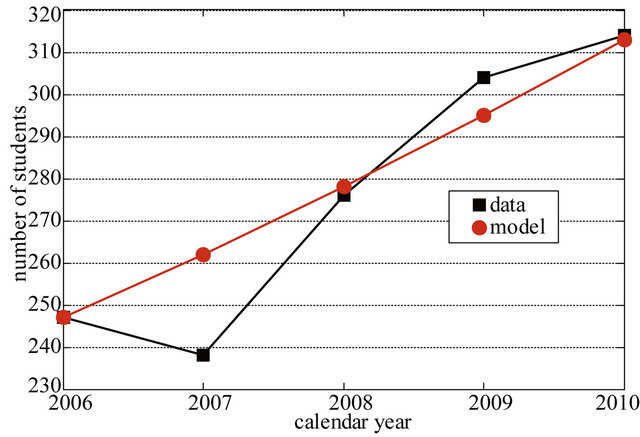
The data of number of students from Department of Mathematics, KMUTNB are collected from student’s data of university. From calendar year 2006 to 2010, the data of changing of number of students are presented in Table 1. The data present number of students for each graduated years which has four years system. The students who remain in the system after four years are included in the fifth year category. The total number of students for each calendar year is focused and plotted in Figure 1. We first observe that the number of students has tendency to increase even though the change in number of freshman has no clear pattern. As seen from Table 1 the data along diagonal shows reduction in number of students from freshmen to the fourth year students. This reduction is due to disqualifying or temporary dropping out.
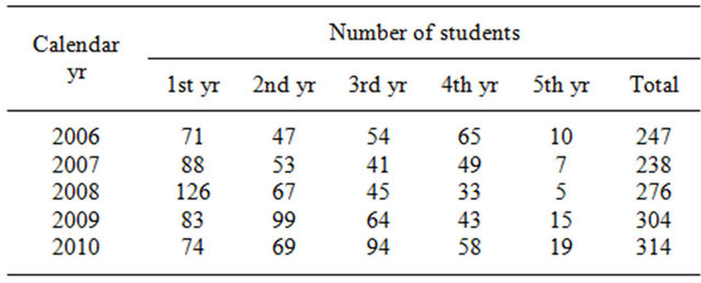
Table 1. Number of students from department of mathematics, KMUTNB from 2006-2010.
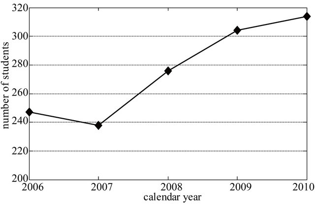
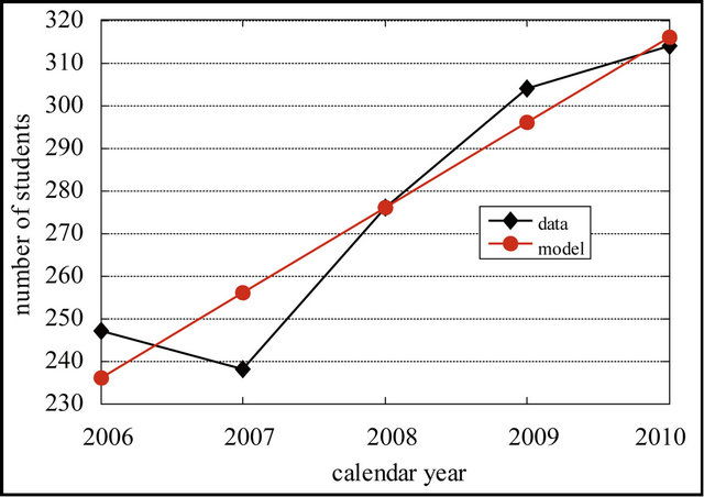
Figure 1. Number of students of Department of Mathematics, KMUTNB from 2006 to 2010.
3. Mathematical Model
In this section, we will formulate the models of number of students using the data from Department of Mathematics, KMUTNB. We present two different kinds of model, i.e., descriptive model and explanatory model. For both models the regression analysis with least square method will be performed according to the data.
3.1. Descriptive Model
Let us define the variable that describes the number of students as  and let
  denote a variable for calendar year. In Figure 1, we observe that the graph of data has a character of straight line. Therefore, we may assume a linear model in the form
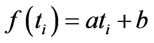 (1)
(1)
where![]() and
and  are parameters that we want to determine and
  denotes data point index. We next estimate the values of parameters
 ![]() and
and  by employing least square method. The sum square error is defined as
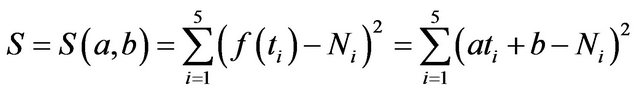 (2)
(2)
Since we need the least of the square of this error, we then differentiate (2) with respect to ![]() and
and  as partial differentiation and rearranging in algebraic equations for
 ![]() and
and  as
as
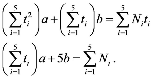 (3)
(3)
Using the data from Table 1, we can compute

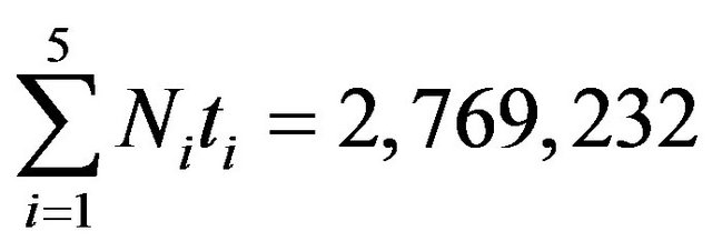
and

Hence, the system (3) becomes
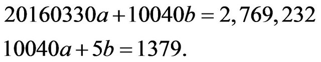 (4)
(4)
By solving (4), we obtain  and
and . Therefore, the linear model is
 . (5)
. (5)
In order to calculate the confidence interval (CI) for parameter ![]() we must compute the standard errors for estimation as
we must compute the standard errors for estimation as
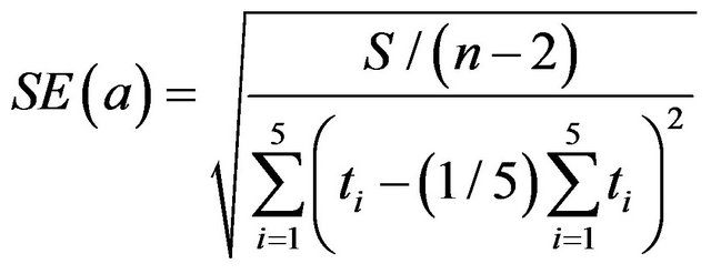 (6)
(6)
where  and
and ![]() is given by (2). Using above formula 95% CI for
is given by (2). Using above formula 95% CI for  is (6.8417, 33.1583). In order to compute 95% CI for predicted model we must provide the standard errors as
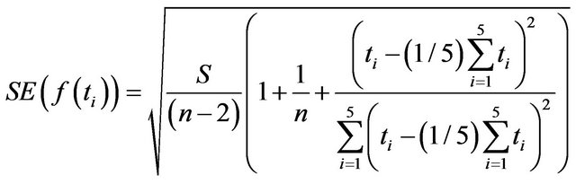 (7)
(7)
Table 2 shows the results of predicting number of students by using the model (5) with percentage error and 95% CI. In Figure 2, the linear model (5) is plotted together with the data.
We next find the square of the correlation coefficient  to consider the percentage of the total variability that is explained by our model. From [4-6]
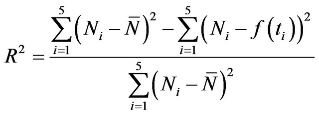 (8)
(8)
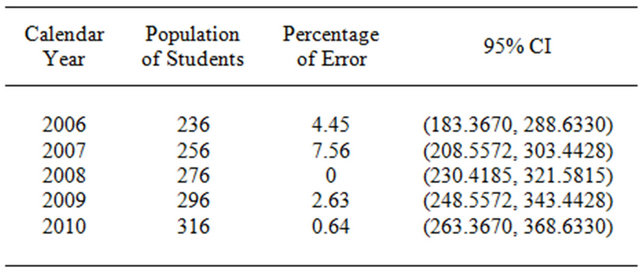
Table 2. The student population predicting from model (5).
we found that 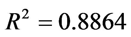 where
where 
and
Therefore, we can claim that the model (5) can explain the data for 88.64%.
3.2. Explanatory Model
From the descriptive model we find how good of the model in predicting the number of students in consecutive year by means of the estimated parameters. However, these parameters cannot provide sufficiently some intuitive information about how changes in population. For example, the model does not reflect the influence of recruitment, graduation or disqualifying from year to year. To address this problem, we consider the mathematical model that can be described such effects in suitable way. We assume that the rates that students are recruited, graduate and moved out from the department are proportional to the number of students and are constant. Therefore, the model can be written in the form
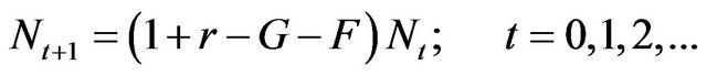 (9)
(9)
where  is number of students at time
 •
•  is the rate at which the first year students enter for each calendar year;
•  is the rate at which the students graduate for each calendar year, and;
•  is the rate at which the students are retired or moving out with any reasons for each calendar year.
It is easy to see that the solution of (9) is given by
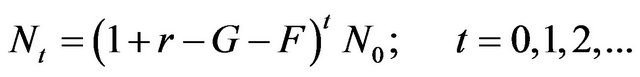 (10)
(10)
Cleary, if , then the number of students will monotonically decrease and vice versa if
 . In order to link model (10) with the data given in section 2, we must determine the parameters
  and
and . By inspecting from the data, we see that the parameters
  and
and  can be estimated in average sense, only parameter
  is unknown. Since we do not have information about the graduation we then attempt to estimate
  by least square method. To this end, we take natural logarithm to equation (10), and thus obtain
 (11)
(11)
where
 . (12)
Since equation (11) is linear, we can use the data from Table 1 to estimate . Providing the estimation for
  and
and  the parameter
  can be obtain from
 . (13)
For the model (10) we set the initial condition as  which is exactly the same value with the first data. Using data in Table 1 we can compute an average recruitment rate and moved out rate as
  and
and . We then transform the data into logarithm function, i.e.
 . After performing the method of least squares with the transformed data set, we are able to estimate
  as
as  where
where  with 95% CI of (0.000138, 0.1177) as shown in Table 3. As in the previous section 95% CI are calculated using the formula (6) and (7). The curve fitting of such data and the values obtained from statistical method is shown in Figure 3.
To see how the model can be used to explain the data we compute the square of the correlation coefficient . Therefore, we can claim that the explanatory model (10) can describe the data for 82.29%.
In order to convert the logarithm to the real function we substitute ,
, ,
, into (13), we then obtain
 . Therefore, the predicting number of students from the explanatory model (10) can be shown in Table 4. Figure 4 shows curve fitting for the original function where
  is defined as 2006,
 ![]() is defined as 2007, and so on.
is defined as 2007, and so on.
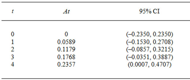
Table 3. Values of  where
where .
.

Figure 3. Curve fitting for the model (11).
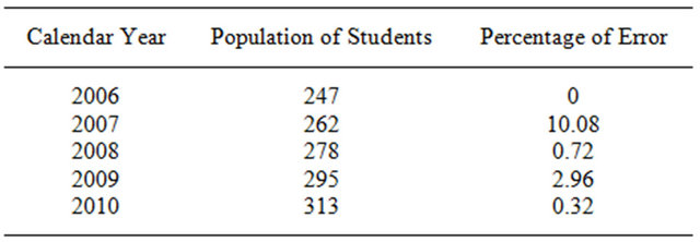
Table 4. The number of students predicting from model (10) with .
.
 ,
,  ,
,  and
and .
.4. Model Application
Regression equation (5) and model (10) can be used toforecast number of students of the Department of Mathematics at KMUTNB in the calendar year 2011. Using model (5) we estimate that the department will have 336 students in 2011, which shows that the number of students will increase 7%. On the other hands, the model (10) predicts 332 students in 2011 which means that the number of students increase 5%. Although the predicted quantity is unknown, what is known about it can be described by a probability distribution, i.e., posterior predictive distribution [7]. Since the regression is approximately linear, then the posterior predictive distribution is approximately  with the parameters mean given by the predicted number of students and the standard errors given in (7), that is

We note that the application is shown only for model (5), the calculation for model (10) is in similar way. Thus, the mean value here is 336. Suppose that the Department administration want to know the possibility that the number of students will increase more than 10% from the last year. We then need to compute
 .
.
To do this, we convert 345 to  value and calculating the tail area. The
  value is
 .
.
Then, we can suggest that there is about 32% chance that the number of student will increase more than 10% from the last year (2010).
5. Conclusions
In summary, the models of student populations of the Department of Mathematics, KMUTNB were constructed. The first model gives linear relationship between the number of students and calendar years while the second model provides nonlinear fashion. Qualitatively, these two models indicate increasing of the number of students. For overall comparison, the coefficient of determinations was calculated and indicates that the descriptive model gives better approximation with respect to the real data than the discrete time model. This shows that the data are likely to be characterized by linear curve given by (1) rather than the nonlinear curve given by (10). Nevertheless, as we pointed out earlier, the second model gives some useful information on how to maintain the the number of students in the future. The results from estimation of parameters in the second model indicate that the freshmen enter the department with the rate close to the sum of moving out and graduation. Thus, the number of students slowly increases. We observe that the graduation rate and moving out of the students have small variation comparing with the recruitment rate. In terms of management, the first two rates could be adjusted by means of action plan while the latter much more depends on outside factors which are difficult to analyze.
Using these models, we can predict the student populations for next calendar year says 2011. Predicting the number of such students for next calendar year is useful for education strategic management and planning of the department such as preparing enough teachers for students coming up next year. In addition, we can use such predictions for course schedule managements. For example, the department can make a decision about the sections or classrooms for the students who will be arriving. Moreover, FTES can be forecasted along with the results from the model. In order to forecast FTES the number of student’s enrollment for each course must be determined by semesters. The forecast FTES would benefit to the evaluation system in both institution and university level.
Finally, the model modification along with alternative method should be considered for future study. For example, instead of using linear fit, one can assume logistic regression or other nonlinear functional forms. We also note that in the second model, the state variable can be structured into more several categories so that the model consists of the number of students for each graduated year. Hence, the transition from year to year could be considered. In such case, the long term data might be also required.
REFERENCES
- R. Q. Lavilles and M. J. B. Arcilla, “Enrollment Forecasting for School Management System,” International Journal of Modeling and Optimization, Vol. 2, No. 5, 2012, pp. 563-566. doi:10.7763/IJMO.2012.V2.183
- S. Choudhuri, C. R. Standridge, C. Griffin and W. Wenner, “Enrollment Forecasting for an Upper Division General Education Component,” Proceedings of the 37th ASEE/ IEEE Frontiers in Education Conference, Milwaukee, 10- 13 October 2007, pp. T3E-25-T3E-28.
- D. Y. Young and L. J. Redlinger, “Modeling Student Flows through the University’s Pipelines,” Proceedings of the 41st Forum of the Association for Institutional Research, Long Beach, 5 June 2001, pp. 1-13.
- J. D. Logan and W. R. Wolesensky, “Mathematical Methods in Biology,” John Wiley & Sons, Hoboken, 2009.
- M. F. Triola, “Elementary Statistics,” Pearson Education, Inc., Boston, 2004.
- R. Peck, C. Olsen and J. L. Devore, “Introduction to Statistics and Data Analysis,” Brooks/Cole Cengage Learning, Boston, 2012.
- G. G. Woodworth, “Biostatistics: A Bayesian Introduction,” John Wiley & Sons, Inc., Hoboken, 2004.
NOTES
*Corresponding author.