Advances in Linear Algebra & Matrix Theory
Vol.4 No.2(2014), Article
ID:45910,14
pages
DOI:10.4236/alamt.2014.42004
New Method of Givens Rotations for Triangularization of Square Matrices
Artyom M. Grigopryan
Department of Electrical and Computer Engineering, The University of Texas at San Antonio, San Antonio, USA
Email: amgrigoryan@utsa.edu
Copyright © 2014 by author and Scientific Research Publishing Inc.
This work is licensed under the Creative Commons Attribution International License (CC BY).
http://creativecommons.org/licenses/by/4.0/


Received 4 March 2014; revised 4 April 2014; accepted 14 April 2014
ABSTRACT
This paper describes a new method of QR-decomposition of square nonsingular matrices (real or complex) by the Givens rotations through the unitary discrete heap transforms. This transforms can be defined by a different path, or the order of processing components of input data, which leads to different realizations of the QR-decomposition. The heap transforms are fast, because of a simple form of decomposition of their matrices. The direct calculation of the N-point discrete heap transform requires no more than 5(N − 1) multiplications, 2(N − 1) additions, plus 3(N − 1) trigonometric operations. The QR-decomposition of the square matrix N × N uses about 4/3N3 multiplications and N(N − 1)/2 square roots. This number varies depending on the path of the heap transform, and it is shown that “the optimal path” allows for significant reduction of number of operations in QR-decomposition. The heap transform and its matrix can be described analytically, and therefore, this transform can also be applied to the QR-decomposition of complex matrices.
Keywords:QR-Factorization, Givens Rotations, Householder Reflections, Heap Transform

1. Introduction
In linear algebra, methods of QR-decomposition (or factorization) of a nonsingular matrix into a unitary matrix and a triangular matrix are well known in mathematics [1] -[3] . QR-decomposition is used in many applications in computing and data analysis. This is the problem of solution of a linear system of equations written in matrix form as . The solution
  can be found after the factorization of the matrix
 , where
  is an orthogonal matrix
  and
and  is a right triangular matrix, in the case when the dimensions of the known vector
 ![]() and unknown
and unknown  are equal. This QR-decomposition is unique if the diagonal coefficients of the matrix
  are positive. In this case,
  , or
, or  in the rank-revealing QR algorithm, when the diagonal elements of the matrix
  are permuted
  in the non-increasing order. There are several methods for computing the QR-decomposition, such as the Gramm-Schmidt process and method of Cholesky factorization. We here mention two other methods: the Householder transformations (known also as Householder reflections) and the Givens rotations. In the second method, each rotation zeros one element in the subdiagonal of the matrix. Therefore, a sequence of
  plane rotations is required for reduction of a square matrix
  to triangular form. The Givens rotations require a large number of arithmetical operations, including multiplications and
  square roots [4] . The method of Householder transforms is the most applied method for QR-decomposition, which reduces the number of square roots to at most
  and uses about
  multiplications [5] -[8] .
In this paper, a new look on the application of Givens rotations to the QR-decomposition problem is described, which is similar to the method of Householder transformations. The concept of the discrete heap transform is applied, which has been introduced in digital signal processing to generate the signal-induced unitary transforms by Grigoryan [9] -[12] . Both cases of real and complex matrices are considered and examples of performing the QR-decomposition of matrices are given. We also illustrate the importance of the path of the heap transform in such decomposition. The traditional way of consequently performing the rotations of data in natural order 1,2,3,... is not the best way, or path, in calculating the QR-decomposition. We briefly describe other more effective paths in QR-decomposition by the heap transforms and give a comparison with the known method of the Householder transformation.
2. Transforms with Decision Equations
Let  and
and  be functions of three variables;
 ![]() is referred to as the rotation parameter such as the angle, and x and y as the coordinates of the point
is referred to as the rotation parameter such as the angle, and x and y as the coordinates of the point  on the plane. These variables may have other meanings. The function
  is parameterized and it is assumed that for a specified set of numbers a and for each point
  on the plane (or its chosen subset) the equation
 (1)
(1)
has a unique solution with respect to![]() . We denote the solution of this equation by
. We denote the solution of this equation by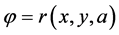 . The system of equations
  is called the system of decision equations. The value of
 ![]() is calculated from the second equation which is called the angular equation. Then the value of
is calculated from the second equation which is called the angular equation. Then the value of ![]() is calculated from the given input
is calculated from the given input  and
and![]() . It is also assumed that the two-dimensional transformation
. It is also assumed that the two-dimensional transformation

which is derived (or whose matrix is calculated) from the given decision equations by  is unitary. These transformations are basic stones to build unitary transforms.
Figure 1 shows the graph of such a basic transformation in part a. The transformation ![]() is defined by given
is defined by given  and
and![]() , namely, the angle
, namely, the angle ![]() is calculated first and then the transform
is calculated first and then the transform  is calculated. The second output is shown with the dash arrow, since the value of this output equals
  which is known from given angular Equation (1). The graph of this transform applied to an input
  is shown in part b.
Example 1: (Elementary rotation). Given a real number , we consider the following functions:
(a) Y-operator (b) X-operator
Figure 1. Graphs of the basic transform  defined (a) by a point
  and applied (b) on an input
 .
.

The basic transformation is defined as a rotation of the point  to the horizontal
![]() ,
,

where the rotation angle ![]() is calculated by
is calculated by  and
and ![]() if
if . The angular equation puts a constrain on parameter a, namely, it is required that
 .
.
3. Discrete Heap Transforms
The composition of the N-dimensional discrete heap transform by a given vector-generator  is performed by the sequential calculation of basic two-dimensional transformations. In matrix form, this composition can be written as follows:
  where each transformation
![]() ,
,  , changes only two components of the input. We assume that the components of an input
  are processed in order
  and
and . This is a natural path
 , and in general, such a path can be taken in many different ways. It is a very important characteristic of the heap transform and the right selection of the path leads to an effective application of the transform in calculating the QR-decomposition. We consider the case, when all basic transformations
 ![]() are parameterized by angles
are parameterized by angles . The special selection of a set of parameters is initiated by the vector-generator
  through the decision equations with a given set of constants
 . The generator is processed first, and during this process all required angles are calculated. For a given set A, we define the following “heap” of elements:

where angles  are calculated by
 ,
,  , and
, and  Thus, it is assumed that the first component of the vector participates in calculations of all
  basic transforms
![]() . As an example, Figure 2 shows the signal-flow graph of determination of the five-point transform by a vector
. As an example, Figure 2 shows the signal-flow graph of determination of the five-point transform by a vector .
.
The N-point transformation  composing from
 ![]() in the space of N-dimensional vectors
in the space of N-dimensional vectors  is defined as

Values of the components ![]() are calculated by
are calculated by

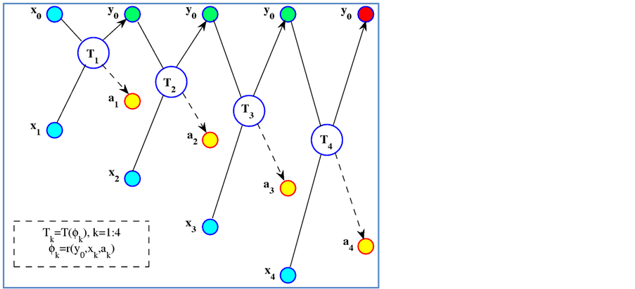
Figure 2. Signal-flow graph of determination of the five-point transform by a vector .
.
where![]() . The first component is transformed sequentially as
. The first component is transformed sequentially as![]() where
where 
 ×××,
×××,  The following should be mentioned about the heap transform. The transform is performed in a space of N-dimensional vectors
 , but all angles
  are found and the transformation
  is composed after solving the decision equations relative to a given vector-generator
 . The transform of
  results in a vector with the constant components of the set A, plus
 ![]() as the first component,
as the first component,

The transformation  is called the N-point discrete
  -signal-induced heap transformation (DsiHT), and the vector
  is the generator of this transformation [6] . The first component
 ![]() is referred to as the heap of the transform.
is referred to as the heap of the transform.
3.1. Transform Collecting Energy
We focus on the special case of the DsiHT, namely on transformations that collect the energy of vectors in one location. The angular equations for such transformations are defined by the set  i.e., when
 ,
, . This condition leads to the fact that the first basis functions of such transforms are the vectorgenerators themselves. Other basis functions are defined based on the correlation data of components of these vectors. Matrices of these transforms are orthogonal. The transforms have simple forms of decomposition that lead to calculation of the N-point transforms with no more than
  multiplications and
  additions.
  operations are also required for calculating elementary trigonometric functions. In the linear space of N-dimension vectors, we construct such an orthogonal transform,
  , whose matrix is defined by
 ![]() where
where  denotes the energy of the vector and
  is the unit vector
 . The term “energy” is referred to as the norm of the vector, i.e.,
 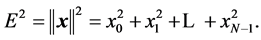 To define the desired transform
 , we consider the following method of energy transferring. Let
  be a 2-D vector to be rotated into a vector
 , i.e.,
The matrix of the transformation,  , which is the Givens rotation, is defined by the matrix equation
 (2)
(2)
The angle ![]() and component
and component ![]() are calculated as
are calculated as ![]() if
if , and
, and
 . If
. If , then
  and
and . The energy is collected in the first components,
 .
.
When processing the N-dimensional vector , the first pair of components,
  , is transferred to the vector
  by Equation (2), as the point
  is rotated to the point
  on the horizontal line. Then, on the next kth step of calculations, when
 , the similar rotations are accomplished over vectors
 , where
 ![]() denotes a new value of the first component on the (k − 1)th step, and
denotes a new value of the first component on the (k − 1)th step, and![]() . The value of the first component
. The value of the first component ![]() is renewed consequently as
is renewed consequently as
 (3)
(3)
where the angles are defined by
 (4)
(4)
Here,  are respectively the matrices of the Givens rotations
 ,
, . As a result, the whole energy of the input signal is collected consequently and, then, transferred to the first component

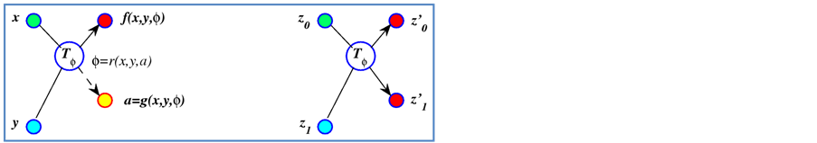
of the transform . Figure 3 shows the signal-flow graph of calculation of the four-point trans-
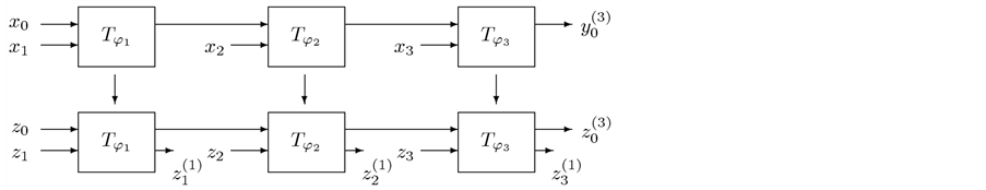
Figure 3.Signal-flow graph of calculation of the four-point heap transform of the vector z.
form of a vector . It is assumed that all parameters
 ,
,  , are calculated by the given vector
  and then used when transforming the vector
3.2. Analytical Expressions
It is important to note, that the basic transformations,  ,
,  , that compose the N-point DsiHT, can be performed without calculation of angles and trigonometric functions. Analytical formulas can be derived for calculation of components of the heap transform
  The matrix of the transform can also be calculated analytically. To show this fact, we introduce the following notations which represent respectively the partial cross-correlation of
  with the vector-generator
  and energy of
 :
:
![]()
where . The components of the heap transform on the kth iteration can be expressed by correlation data as
 (5)
(5)
On the final step, the value of the first component is defined by  which is the correlation coefficient of the input signal
  with the normalized signal-generator
 . In the particular
  case, we obtain
  and the rest of coefficients
 .
.
The coefficients  of the matrix of the N-point DsiHT can be obtained from equations in (5). The mth row of the matrix of the transform is defined by applying the unit vector
  with 1 on the mth position, where integer
 . Therefore, the coefficients can be calculated as
 (6)
(6)
4. Transforms with Decision Equations
In this section, we give a brief analysis of the matrix decomposition by the heap transformations and the comparison with the known methods which are based on rotations in two dimensions. It should be noted first that the discrete heap transformations differ from the well-known Householder transformation [2] , whose matrix  is symmetric and defined as
 , where the normalized vector
  is calculated

and  is a given vector. For example, when
 , the Householder vector equals
  and the matrix of the Householder transform is
The matrix of the heap transformation generated by the same vector x equals
These two transformations result in the same vector,  , where
 . Both transformations have the same first basis function which equals the normalized vector-generator.
The heap and Householder transformations differ much when considered with the large dimensions. For instance, when ![]() and the vector-generator
and the vector-generator , we obtain the following symmetric matrix of the Householder transformation with determinant one:
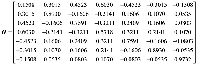
and the vector  The orthogonal matrix of the heap transformation generated by the vector
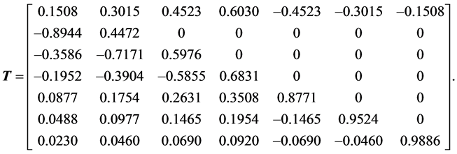
  is not full filled and has the zero upper triangular submatrix with 15 zeros,
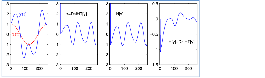
We now illustrate the difference of the DsiHT and Householder transforms applied on signals. Figure 4 shows the example with the 257-point signal  and noisy signal
 in part a, along with the
  -induced heap and Householder transforms
 (a) (b) (c) (d)
Figure 4. (a) The original  and signal
  with a random noise, (b) the 257- point discrete heap transform of
 , (c) the 257-point Householder transform of
 , and (d) the point wise difference of these transforms.
of  respectively in b and c, and the difference of these two transforms in d. The first seven values of the Householder and heap transforms are the following:
 22.6276, −1.0608, −1.0285, −0.9915, −0.9503, −0.9052, −0.8568,
![]() 22.6276, 0.0190, 0.0366, 0.0566, 0.0788, 0.1031, 0.1291.
22.6276, 0.0190, 0.0366, 0.0566, 0.0788, 0.1031, 0.1291.
The big difference of these transforms occurs in the first ninety components.
5. Matrix Decomposition
We now consider the application of heap transforms for calculating the determinant of a nonsingular square matrix, as well as its decomposition. The method described in this section is based on the same idea as the method of Householder transforms, also known as the Householder reflections. Although the heap transformation and Householder transformation are different, it is evident that these two concepts should result in the same (or similar) decomposition, but by different ways.
Let  be a real square matrix (N × N) with
 . We denote coefficients of this matrix as
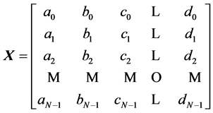 .
.
Let vector  be the first column of this matrix,
 . We denote by
 ![]() the matrix of the heap transformation
the matrix of the heap transformation ![]() generated by this vector. This matrix contains an upper triangular submatrix with
generated by this vector. This matrix contains an upper triangular submatrix with  zeros. The product of two matrices
  results in a matrix
  with the first column equal to
 . Therefore, the matrix
  has the following form:
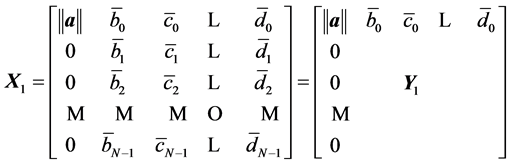
where we denote by  the
the  minor of this product. We can repeat the described above process for the submatrix
 , by considering its first vector-column
  as a generator for the
  - point heap tranformation
 , whose matrix we denote by
![]() . The product of two matrices
. The product of two matrices

is a matrix (N × N) with the second column equal

On this step, the matrix  is transformed to the matrix
  which has the following form:
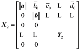
where ![]() is the (2,2) minor of this product and has the size
is the (2,2) minor of this product and has the size 
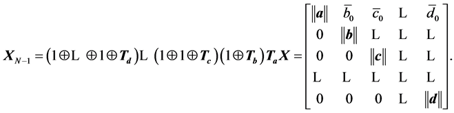
On the next step, we consider the first vector c of the submatrix ![]() and construct the matrix
and construct the matrix ![]() of heap transformation generated by
of heap transformation generated by . Then, the (3,3) minor
 ![]() of the product of the matrices
of the product of the matrices

is transformed into a matrix whose the first column is zero, except in the first row. The process of such transformations is repeated until we obtain the upper triangular matrix:
The determinant of the matrix equals , since all heap transformations have determinant one. Thus, the determinant of a square nonsingular matrix can be calculated by using the heap transforms. We denote by
  the product of the following matrices

Each heap transformation is unitary, and R is unitary. The inverse matrix  can thus be represented by
![]()
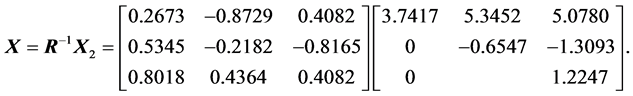
We obtain the following decompositions of the matrix  and its inverse:
 ,
,  , where
  and
and  are the upper triangular matrices, and
  is unitary.
Example 2: Consider the decomposition of the following matrix (3 × 3):

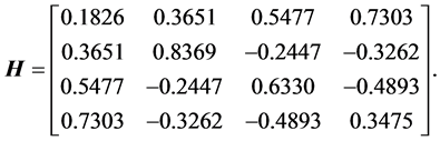
The decomposition of  by the heap transforms,
  , results in the unitary matrix
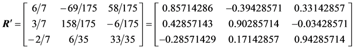
and the upper triangular matrix
The coefficients of the matrix ![]() are given with precision of eight digits after the point. The decomposition of the matrix
are given with precision of eight digits after the point. The decomposition of the matrix  by the Householder transforms is defined by the same matrices,
  and
and . Thus, by means of the heap transforms which are composed by the Givens rotations, we achieve the same decomposition as the Householder reflections. It should be noted, that the first row-vector of the matrix
  equals to the normalized first column-vector
  of the original matrix
 . For the example considered above, we obtain

Arithmetic Complexity of the Decomposition
The  -generated heap transform of a vector
  can be calculated by using analytical Equations (5) and (6),
 (7)
(7)
The calculation of all energy coefficients ,
,  , requires
 ![]() multiplications. The total number of multiplications is calculated by
multiplications. The total number of multiplications is calculated by , plus
 ![]() square roots. When the matrix
square roots. When the matrix  is multiplying by another square matrix, the number of required multiplications can be calculated as
  plus
plus ![]() square roots. If we use this estimation to calculate the number of multiplications for factorization of a square nonsingular matrix by heap transforms, we obtain the following number:
square roots. If we use this estimation to calculate the number of multiplications for factorization of a square nonsingular matrix by heap transforms, we obtain the following number:

plus  square roots.
6. Strong Heap Transform
The point, or the heap, where the energy of the vector-generator is transferred is not required to be at the first location of the signal. The DsiHT can be defined by equation ![]() for any unit vector
for any unit vector . The path P along which we compose the heap is important, not a location of energy integration, when defining the discrete heap transform. As an example, we consider the basic transforms that sequentially process the last pair of components of the signal. This is the case, when the path P of the heap transformation induced by a vector-signal x is defined as
 ,
, . We call this heap transformation the strong heap transformation. The energy from each component xk is taken away and given to the last component
 . The strong heap transformation generated by the vector x results in the transform
 .
.
Example 3: For the vector , the matrix of this heap transformation is orthogonal and equals

It is interesting to note that the energy of the signal is transferred sequentially to the first component in numbers 5, 5.3852, and 5.4772. This heap of numbers is smaller than the numbers 2.2361, 3.7417, and 5.4772, when the four-point DsiHT is composed along the ordinary path ,
,  , by Equations (3) and (4). That can be explained because of small values of the first components of the signal
 .
.
The method of triangularization of a square nonsingular matrix  by the strong heap transformations is described similarly to the method described in Section 4 for the ordinary path. The only difference is that on each kth step of calculations, where
 , the generator of the strong heap transformation, which is zeroing the kth column of the renewed matrix
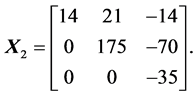
 , is taken from the top part of the column. To illustrate this method, we consider the matrix
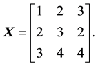
The first column  generates the strong heap transformation whose matrix equals

and . The product of matrices
 ![]() and
and  equals

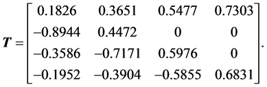
Continuing zeroing the first two elements of the second column of this matrix, by using the strong heap transformation defined by the vector , we obtain the following decomposition of the matrix
  by the product of the unitary matrix
 ![]() and the lower triangular matrix
and the lower triangular matrix :
:
 (8)
(8)
The determinant of  can be calculated as
 . Thus, we obtain the decomposition of the square matrix
  by the product of the unitary matrix
 ![]() and lower triangular matrix
and lower triangular matrix . It should be noted for the comparison that when using the ordinary path,
  ,
,  , the following decompositions of the matrix
  holds:
It is evident that there is a relation between this decomposition and the decomposition of Equation (8). The first and third columns of the matrices ![]() have been rearranged, as well as the first and third rows of the matrices
have been rearranged, as well as the first and third rows of the matrices . In addition, the signs of the second column of
 ![]() and second row of
and second row of  have been changed. Many operations can be saved in the different steps of calculation of the QR-decomposition, if we learn how to select an optimal path in the heap transform. The optimality relates to minimization of the computation complexity of the QR-decomposition.
Optimal Path of the DsiHT
The path of the heap transformation is an important characteristic of the transformation. In the described above method of QR-decomposition of the matrix by the heap transformations, the ordinary path and path for the strong heap transforms were used. For effective decomposition of non-singular matrices, other well-considered paths  may lead to effective matrix decomposition. The finding such optimal paths is therefore desirable. To illustrate the importance of the path in the heap transformation, we consider the following example with the seven-dimensional vector-generator
  The heap transformation with this generator is defined by the following six steps of calculations (or Givens rotations):
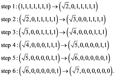
The calculations require six different square roots. Each component of the vector, except the first one, is processed only ones. We now consider another path  in the heap transformation, which is shown in Figure 5 where the first column corresponds to the generator.
In this path, the transformation rounds three times the components of the input and intermediate data, and on each round a certain number of heaps are calculated, which then are transferred to one heap. During the first round, three different pairs of components ,
,  , and
, and  are processed separately and three heaps of value
  each are calculated, as shown in the second column. Component
  is not used in this stage since the dimension of the input is 7, odd number. In the second round, the first three obtained outputs together with
  are used to calculate two heaps with values of
  and
and . In the last round, these two heaps are rotated to collect the whole energy
  in one heap. The calculation of the heap transform by the path
  is thus described by six Givens rotations as follows:
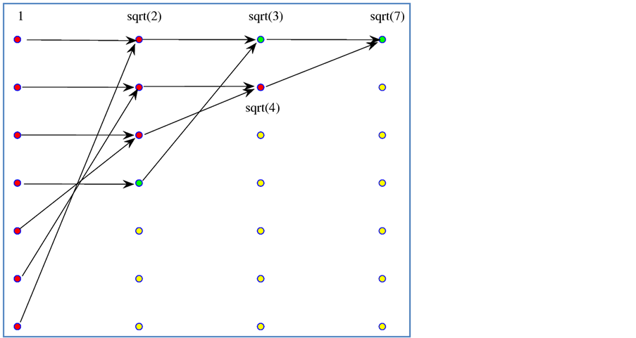
Figure 5. Signal-flow graph of the seven-point heap transformation H .
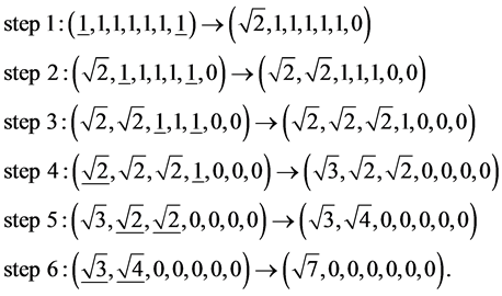
The underlined numbers in the input vectors show the pairs which are used in rotations in each step of calculation. The same number, six, of steps are used to accomplish the heap transform , however there are only four different square roots are calculated,
  , and
, and . We can also define such a path for the general
 ![]() case, by composing first the transformation on the first round as
case, by composing first the transformation on the first round as

where  is the integer part of
  and
and ![]() is the empty operator if
is the empty operator if ![]() is even, and the identity operator if
is even, and the identity operator if ![]() is odd. The transformations
is odd. The transformations  are the Givens rotations of two components of a vector with numbers
 ![]() and
and , when
 . On the next round, the transform over the first half of outputs is composed similarly,
 . Continuing this process of transformation until the last round which is completed by the transformation
 , we obtain the following heap transformation:
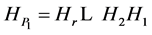 . The number
  of rounds in the path
  equals the closest integer to
 .
.
Example 4: Let  be the vector
 . The signal-flow graph of the heap transformation generated by
  with path
  is given in Figure 6.
The orthogonal matrix of this transformation equals
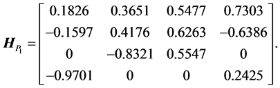
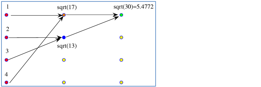
Figure 6. Signal-flow graph of the four-point heap transformation ![]() by the path
by the path .
.
For comparison, we consider the matrix of the heap transformation defined by the ordinary path ,
,

Both transformations result in the same vector, . The matrix
 ![]() has four zero coefficients which are located symmetrically, and
has four zero coefficients which are located symmetrically, and  has three zeros composing a triangle.
Example 5: Let  be the vector
 . The signal-flow graph of the heap transformation generated by
  is given in Figure 5. The orthogonal matrix of this transformation equals
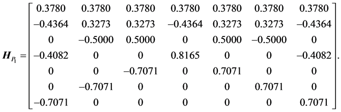
This matrix is symmetric with respect to the middle column, and it has one triangle in the center, which is fully filled by zeros. We also can see two not fully filled by zeros triangles in both sides of the middle column. There are total 22 zeros in these triangles, more than in the matrix of the heap transformation defined by the path P. Indeed, the matrix of this transformation equals
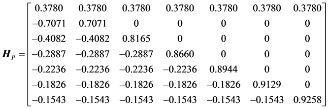
with 15 zero coefficients. Since the matrix ![]() is sparse the application of the heap transformations with the path
is sparse the application of the heap transformations with the path  leads to the effective QR-decomposition of non-singular matrices. Indeed, in each step of the decomposition, the use of the heap transformation by the path
  requires fewer operations, when compared with the heap transformation by the path
 , for large dimensions
![]() . The matrix of the first transformation is sparser than the second one. For instance, in the (5 × 5) example, total 14 multiplications can be saved when using the paths
. The matrix of the first transformation is sparser than the second one. For instance, in the (5 × 5) example, total 14 multiplications can be saved when using the paths  in the QR-decomposition of the matrix
  instead of
  path.
path.
7. Complex DsiHT
In this section, we describe briefly the case when heap transforms are generated by complex vectors and applied on complex vectors. For that we stand on Equation (7) which allows for defining the complex version of the heap transformation. Indeed, we can apply these equations wherein the correlation data are calculated as follows:
![]()
Here, the bar denotes the operation of the complex conjugate. The transformation defined by these equations is unitary and is called the complex heap transformation. The basic two-dimensional transformation T, which is defined by a complex vector , and then, is applied to a complex input
  is calculated in matrix form as follows:

When , we obtain the real transform
  It should be noted that this transformation differs from the known definition of the complex Givens rotation [4] , whose matrix is calculated as
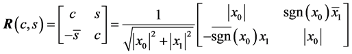
where the complex sign function is defined by . This rotation results in the following complex transform
  where
where  is a complex number with norm one.
Example 6: Let ![]() and let the complex vector
and let the complex vector  to be
to be . The complex heap transformation generated by this vector has the following matrix:

The transform of the vector-generator equals , where
 . The matrix
  is the complex conjugate to
  and its first row is the normalized generator, i.e.,
  . The complex heap transformations can be used for triangularization of the square complex matrix in a way similar to the real case described above. As an example, we consider the following matrix:
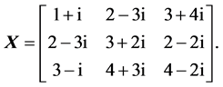
The method of heap transforms results in the following decomposition of  where
where  is the unitary matrix
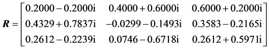
and  is the upper triangular matrix

8. Conclusion
A novel decomposition of nonsingular real and complex matrices by fast heap transforms has been described, when the paths  of the transforms are natural. The path of the heap transform is an important characteristic of the transform, and other paths
  can be found, that may result in more sparse matrices than the path
  does. The application of such paths will lead to effective matrix decomposition, as shown on examples with the strong heap transform. We have considered only the case of nonsingular matrices of square size. However, the calculations presented above can be applied to the case of non square matrices, as well.
References
- Horn, R.A. and Charles, R.J. (1985) Matrix Analysis. Cambridge University Press, Cambridge. http://dx.doi.org/10.1017/CBO9780511810817
- Moon, T.K. and Stirling, W.C. (2000) Mathematical Methods and Algorithms for Signal Processing. Prentice Hall, Upper Saddle River.
- Morrison, D.D. (1960) Remarks on the Unitary Triangularization of a Nonsymmetric Matrix. Journal ACM, 7, 185-186. http://dx.doi.org/10.1145/321021.321030
- Golub, G.H. and Van Loan, C.F. (1996) Matrix Computations. 3rd Edition, Johns Hopkins, Balimore.
- Householder, A.S. (1958) Unitary Triangulation of a Nonsymmetric Matrix. Journal ACM, 5, 339-342. http://dx.doi.org/10.1145/320941.320947
- Anderson, E., Bai, Z., Bischof, C.H., et al. (1999) LAPACK Users’ Guide. 3rd Edition, SIAM Philadelphia, Philadelphia. http://dx.doi.org/10.1137/1.9780898719604
- Bindel, D., Demmel J., Kahan, W. and Marques, O. (2001) On Computing Givens Rotations Reliably and Efficiently. LAPACK Working Note 148, University of Tennessee, UT-CS-00-449.
- Demmel, J., Grigori, L., Hoemmen, M. and Langou, J. (2012) Communication-Optimal Parallel and Sequential QR and LU Factorizations. SIAM Journal on Scientific Computing, 34, 206-239. http://dx.doi.org/10.1137/080731992
- Grigoryan, A.M. and Grigoryan, M.M. (2006) Nonlinear Approach of Construction of Fast Unitary Transforms. In: Proceedings of the 40th Annual Conference on Information Sciences and Systems (CISS 2006), Princeton University, Princeton, 1073-1078. http://dx.doi.org/10.1109/CISS.2006.286625
- Grigoryan, A.M. and Grigoryan, M.M. (2007) Discrete Unitary Transforms Generated by Moving Waves. Proceedings of the International Conference: Wavelets XII, SPIE: Optics + Photonics 2007, San Diego.
- Grigoryan, A.M. and Grigoryan, M.M. (2007) New Discrete Unitary Haar-Type Heap Transforms. Proceedings of the International Conference: Wavelets XII, SPIE: Optics + Photonics, 6701.
- Grigoryan, A.M. and Grigoryan, M.M. (2009) Brief Notes in Advanced DSP: Fourier Analysis with MATLAB. CRC Press, Taylor and Francis Group, Philadelphia.