Modeling and Numerical Simulation of Material Science
Vol.3 No.2(2013), Article ID:30785,12 pages DOI:10.4236/mnsms.2013.32007
The Interlaminar Stress of Laminated Composite under Uniform Axial Deformation
1Beijing Institute of Mechanical Equipment, Beijing, China
2Shanghai Jiao Tong University, Shanghai, China
Email: jbchen@sjtu.edu.cn
Copyright © 2013 Chuijin Yang et al. This is an open access article distributed under the Creative Commons Attribution License, which permits unrestricted use, distribution, and reproduction in any medium, provided the original work is properly cited.
Received November 27, 2012; revised December 28, 2012; accepted January 11, 2013
Keywords: Interlaminar Stresses; Finite Element Method; Laminated Composite Plate
ABSTRACT
The interlaminar stresses are analyzed by combining the first shear theory with the layerwise theory method. And the plate subjected to a uniform axial strain is studied by the simplified displacement field. Using the simplified displacement field, the equations of finite element method are developed by the principle of virtual work. And the amount of calculation is reduced by using the linear element. Then, some numerical examples are given to verify the accuracy of the method and analyze the distribution of interlaminar stresses along y-axis and z-axis. The shapes of the stresses’ curves in the vicinity of the free edge are very different from the interior area. Moreover, the influence of the ply angle on the interlaminar stresses is analyzed for the plate [θ/−θ]s. It can be found that the shapes of the stresses along z-axis are similar when the angle is different, while the values of the interlaminar stresses are changed apparently with the ply angle.
1. Introduction
The composite materials are widely used in the aviation, space industries and mechanical engineering because of their good command of mechanical property. The laminated composite plate is made up of multilayer lamination. Their interlaminar stresses can significantly contribute to delamination even when they are much lower than the failure strength of the classical lamination theory. They may make the potential of laminated composite plate can not be worked out for its carrying capacity deteriorated because of the delamination. In the vicinity of the free edge, the interlaminar stresses are varied fast, which is the main reason of delamination. And the delamination of the laminated composite plates is the most common destruction form of laminated composite plates. Therefore, the research of interlaminar stresses is of great significance to practical applications. Many researchers have done a lot of work about it. The stresses in the vicinity of free edge are expressed as a two-dimensional state by the classical lamination theory [1,2]. Afterward, it was proved to be a three-dimensional state by many researchers [3-5]. In recent 10 years, many more people have started to research the interlaminar stresses. Hiroyuki Matsunaga analyzed the stresses and displacements in the laminated composite beams subjected to lateral pressures by using the method of power series expansion of displacement components [6]. Asghar Nosier and Arash Bahrami studied the interlaminar stresses in antisymmetric angle-ply laminates by developing a reduced form of displacement field for long antisymmetric angle-ply composite laminates subjected to extensional and/or torsional loads [7]. Theofamis S. Plagianakos and Dimitris A. Saravanos proposed a higher-order Layerwise theoretical framework to calculate the static response of thick composite and sandwich composite plate [8]. The displacement field they assumed in each discrete layer included quadratic and cubic polynomial distributions of in-plane displacements. Furthermore, a Ritz-type exact solution [8] was implemented to yield the structural response of thick composite and sandwich composite plates. Heung Soo Kim et al. developed a stress functionbased variational method to investigate the interlaminar stresses near the dropped plies [9]. M. Amabili and J. N. Reddy developed a consistent higher-order shear deformation non-linear theory for shells of generic shape [10]. Using the developed theory, a simply supported, laminated circular cylindrical shells subjected a large amplitude force vibrations are studied. Amir K. Miri and Asghar Nosier investigated free-edge effects in antisymmetric angle-ply laminated shell panels under uniform axial extension by using layerwise theory [11]. And the problem was analytically solved for specific boundary conditions along the edges. Ren Xiaohui et al developed a higher-order zig-zag theory for laminated composite and sandwich plates [12]. The proposed theory can predict more accurate in-plane displacements and stresses in comparison with other zig-zag theories. J. L. Mantari et al. developed a new shear deformation theory for sandwich and composite plates [13]. The proposed displacements field was assessed by performing several computations of the plates governing equations and the results were relatively close to 3D elasticity bending solutions.
The first shear theory is combined with the Layerwise theory (LWT) [14] to analyze the interlaminar stresses of the laminated composite plates in this paper. The first shear theory assumed the plate as an equit-single layer as to build the displacement field whose component is C0 continuity. The Layerwise theory builds the displacement field by dispersing the plate to many numerical layers. In this paper, the interlaminar stresses are analyzed by superimposed the first shear theory on the Layerwise theory. Then, the displacement field is simplified for the symmetric ply composite plate which subjected to a uniform axial strain. The finite element equation is derived by the principle of virtual work. Then, the linear element is used to solve the problem. Of course, it reduced the amount of calculation while the accuracy is ensured. At last, the results of the interlaminar stresses are given for different ply conditions of laminated composite plates.
2. The Displacement Field
Superimposing the first shear theory on the Layerwise theory, the displacement field can be expressed as:
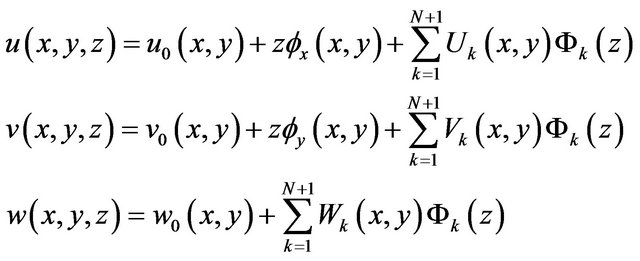 (1)
(1)
where, N is the number of numerical layers through the thickness. 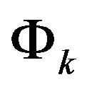 is the global interpolation function which is linear or quadratic Lagrange interpolation function in general. And the discretization of the displacements is fulfilled by it (see Figure 1).
Considering the plate which is symmetric plied and subjected to a uniform axial strain (see Figure 2), the displacement field can be simplified as:
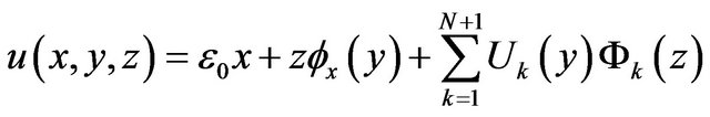
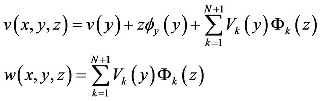 (2)
(2)
where,  is the uniform strain along x-axis and the displacement v is independent of variable x. Therefore, this situation can be solved as the problem of plane strain.
In this paper, the linear Lagrange interpolation function [14] is used as the interpolation function , and it can be expressed as below [14]:
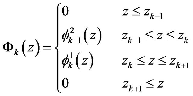 (3)
(3)
where, 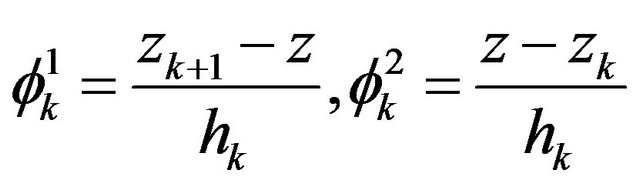 , and hk is the thickness of the kth layer. The displacement field adopted here is satisfied the displacement continuity condition and the shear stresses continuity condition between layers.
3. The Finite Element Equation
Considering the laminated composite plate which is symmetric plied and subjected to a uniform axial strain along x-axis. Substitute Formula (2) into the principle of virtual work as below:
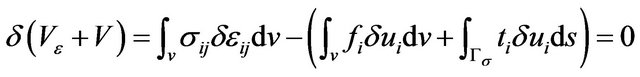 (4)
(4)
Then the finite element equation can be derived and wrote simply as:
 (5)
(5)
where, K is the element stiffness matrix, d represents the displacement vector of element node and F represents the nodal load vector. The definite expression of the finite element equation can be seen in the appendix at the
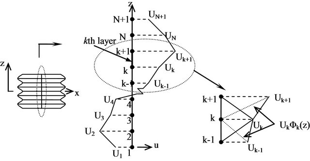
Figure 1. The discretization of displacements through the thickness.
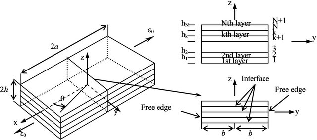
Figure 2. Geometrical model.
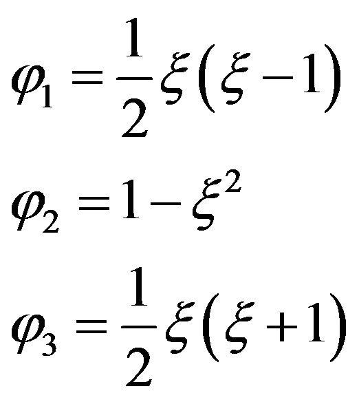
end of this paper. It should be noticed here that the element stiffness matrix in Formula (5) is unsymmetric, which is different from the general finite element equation. Here the Lagrange element with 3 nodes (see Figure 3) is applied to solve the problem as  is used to interpolate the displacements along z-axis, which simplify the deducing process of finite element equation. Using the nature coordinates, the interpolation shape function can be expressed as below:
 (6)
(6)
where,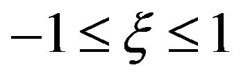 .
.
The results at the Gauss points have the highest accuracy because of the Gauss integral is used in the calculation process. Therefore, the stresses at the Gauss points are used to plot the curves in this paper. It should be noticed that the results of the nodes which connect two different elements are not equal in the two elements.
4. Numerical Results
A symmetric plied composite plate subjected to a uniform axial strain  is studied here. And its length, width and height are 2a, 2b and 2h respectively (see Figure 2). At the same time, it is assumed that each material layer is orthotropic and equal thickness. And the elasticity modulus, shear modulus and Poisson’s ratio are as follows:
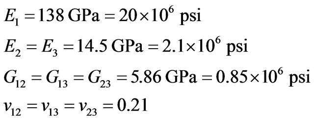 (7)
(7)
where the subscripts 1, 2, 3 represent the three principal axis of the material, and 1 psi = 6.895 kPa. The 1/8
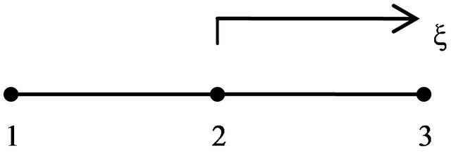
Figure 3. The Lagrange element with 3 nodes.
model is studied here as the laminated composite plate is assumed to be symmetrical about the x-y plane and z-axis. As to compare the results of this paper with the results of other researchers, the stresses are normalized as below:
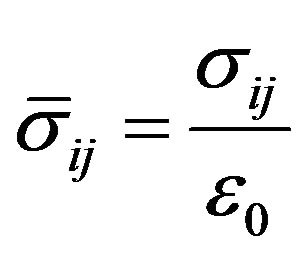 (8)
(8)
4.1. Cross Ply Laminates: [0/90]s and [90/0]s
4.1.1. The Stresses along y-Axis
The distributions of stresses (σz, σxz, σyz) along y-axis at z = 0 and z = h/2 of the cross-ply laminated composite plate ([0/90]s) are shown in Figures 4 and 5. The results are in accordance with the quasi-3D element method [15]. As shown in the Figures, At the interface z = 0 or z = h/2, σz grows fast near the free edge. Meanwhile, σxz is very close to zero which is same as the theoretical result. And the stress σyz approaches to zero gradually in the vicinity of the edge, which is accordance with the boundary condition that σyz is zero at the edge.
The distributions of stresses (σz, σxz, σyz) along y-axis at z = 0 and z = h/2 of the cross-ply laminated composite plate ([90/0]s) are shown in Figures 6 and 7. It can be seen that σz and σyz grow fast in the vicinity of the edge, while the value of σxz is zero at the edge.
It can be observed that the failure of material is occurred easily in the vicinity of the free edge of the crossply laminated composite plate.
4.1.2. The Stresses along z-Axis
The distributions of stresses (σz, σxz, σyz) along z-axis of the cross-ply laminated composite plate ([90/0]s) are shown in Figures 8-10. It can be observed that the values of the stresses are zero on the surface. The interlaminar
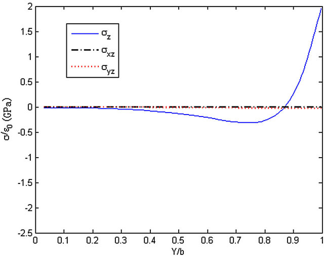
Figure 4. The stresses along y-axis, z = 0, ([0/90]s).
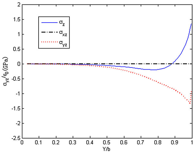
Figure 5. The stresses along y-axis, z = h/2, ([0/90]s).
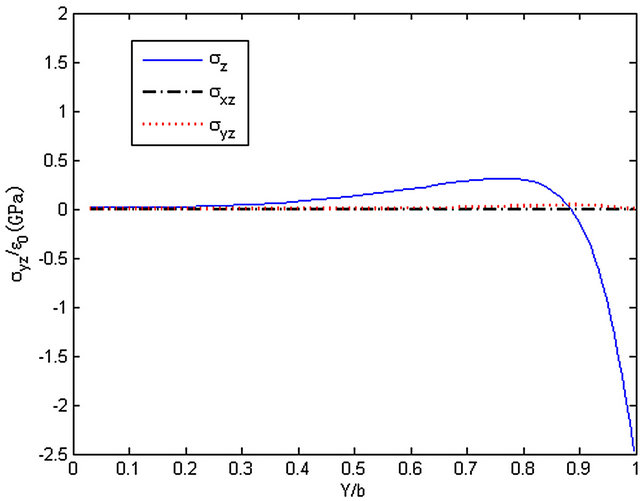
Figure 6. The stresses along y-axis, z = 0, ([90/0]s).
stresses at the cross section y = 0.25b are almost same as y = 0.5b. Along z-axis, the stress σz grows slowly and reaches the maximum at y = 0. The stress σxz is close to zero and hardly change. Besides, the stress σyz reaches a
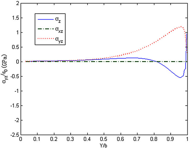
Figure 7. The stresses along y-axis, z = h/2, ([90/0]s).
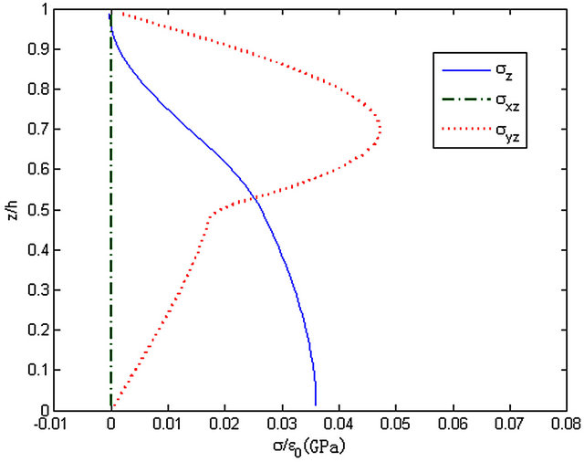
Figure 8. The stresses along z-axis, y = 0.25b.
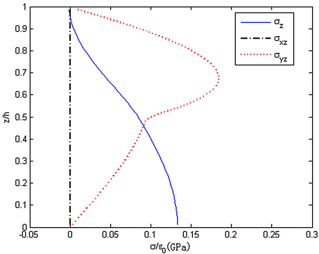
Figure 9. The stresses along z-axis, y = 0.5b.
peak near the interface z = 0.7h and it changes suddenly at z = 0.5h, while its value is close to zero at z = 0. At the cross section y = 0.99b, stress σz changes from tension to pressure suddenly at the interface z = 0.5h. Like σz, stress σyz changes from pressure to tension suddenly at z = 0.5h while its value is close to zero when z = 0. Besides, it can be observed from the three figures that the stresses are much higher when y = 0.99b than the others. It means that the stresses are much higher near the free edge than the interior area. And the destruction is easier to be happened in the vicinity of the free edge.
4.2. Angle Ply Laminates: [45/-45]s
4.2.1. The Interlaminar Stresses along y-Axis
The results of the interlaminar stresses of the laminated composite plate ([45/-45]s) are shown in Figures 11 and 12. It can be observed that σz grows very fast in the vicinity of the edge while a minimum is happened at the edge. Stress σyz reaches a peak in the vicinity of the edge followed a sharp decreased. It is different from the elastic solution proposed by Wang and Choi which shows that stress σyz is vanished at the edge. Stress σxz grows as a
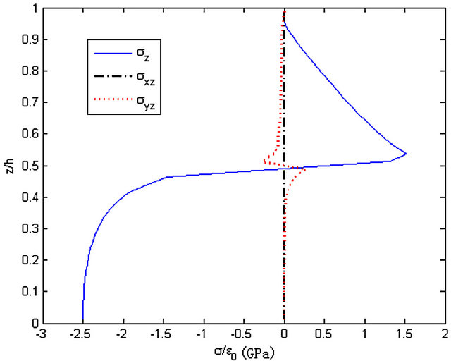
Figure 10. The stresses along z-axis, y = 0.99b.
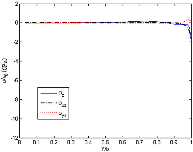
Figure 11. The stresses along y-axis, z = 0.
smooth curve along y-axis and reaches a maximum at the edge.
4.2.2. The Interlaminar Stresses along z-Axis
The distributions of stresses (σz, σxz, σyz) along z-axis of the cross-ply laminated composite plate ([45/-45]s) are shown in Figures 13-15. It can be observed that the val ues of three stresses are zero on the surface. And at the cross sections y = 0.25b and y = 0.5b, the distributions of interlaminar stresses are similar. Both the three stresses take a sharp turn at the interface of the cross section y = 0.99b. Stress σyz changes from tension to pressure while stresses σz and σxz reach a sharp peak at z = 0.5h. It also can be seen that the value of the stresses near the free edge is much higher than the stress at the interior area.
4.3. Angle Ply Laminates: [45/-45/0/90/90/0/-45/45]s
4.3.1. The Stresses along y-Axis
The distributions of stresses (σz, σxz, σyz) along y-axis of
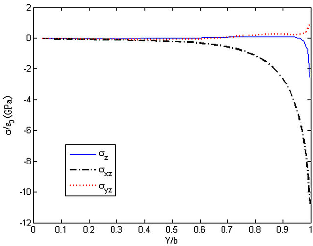
Figure 12. The stresses along y-axis, z = h/2.
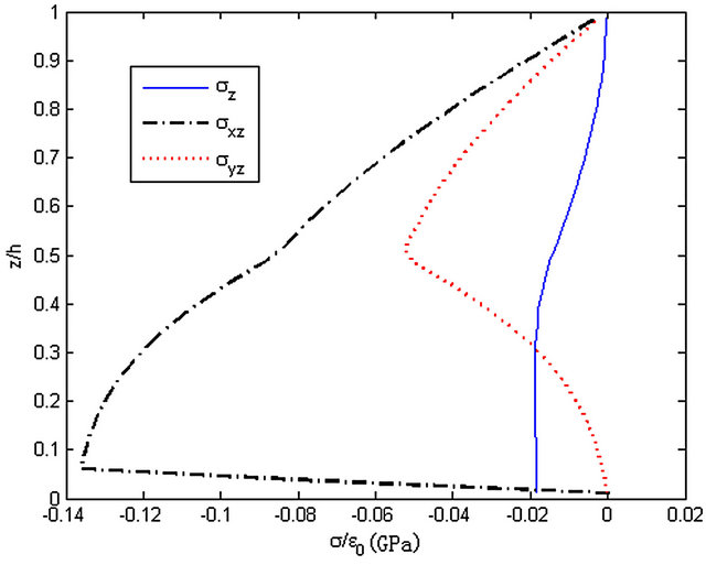
Figure 13. The stresses along z-axis, y = 0.25b.
the angle ply laminates ([45/-45/0/90/90/0/-45/45]s) are shown in Figures 16-23. It can be observed that the curves of the stresses change sharply in the vicinity of
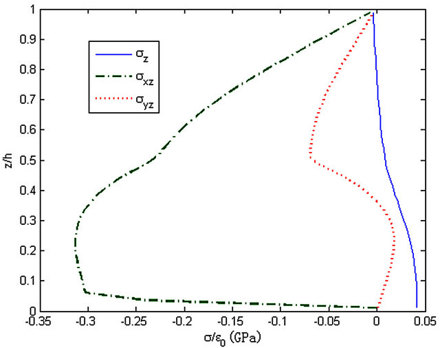
Figure 14. The stresses along z-axis, y = 0.5b.
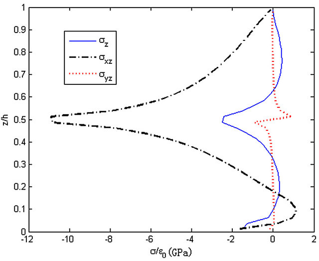
Figure 15. The stresses along z-axis, y = 0.99b.
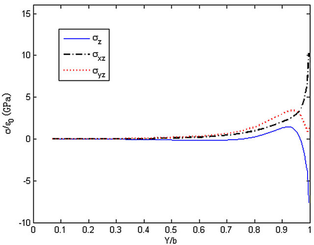
Figure 16. The stresses along y-axis, z = 0.
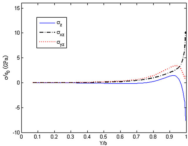
Figure 17. The stresses along y-axis, z = h/8.
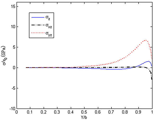
Figure 18. The stresses along y-axis, z = h/4.
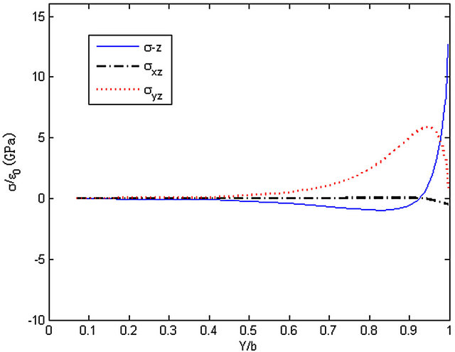
Figure 19. The stresses along y-axis, z = 3h/8.
the edge. Stress σyz reaches a peak near the edge then to zero while stress σz and σxz both reach a maximum or minimum at the edge.
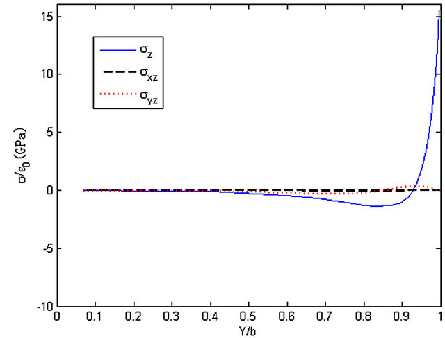
Figure 20. The stresses along y-axis, z = h/2.
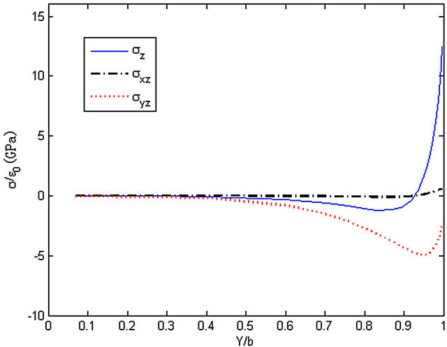
Figure 21. The stresses along y-axis, z = 5h/8.
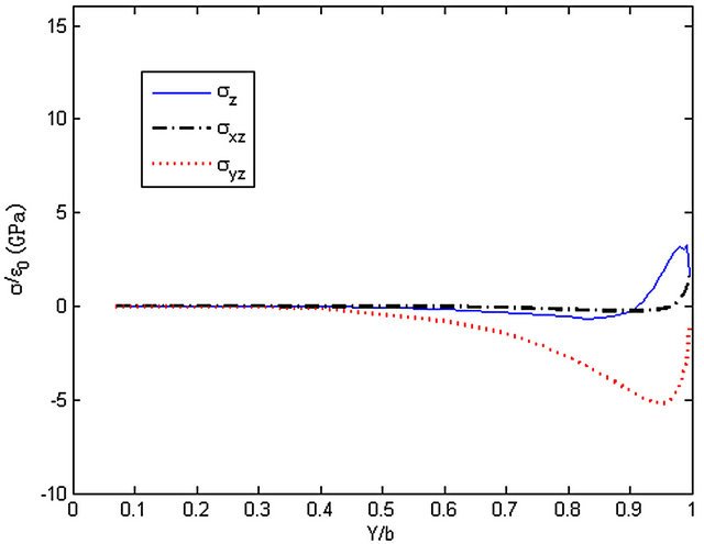
Figure 22. The stresses along y-axis, z = 3h/4.
4.3.2. The Stresses along z-Axis
The distributions of stresses (σz, σxz, σyz) along z-axis of the angle ply laminates ([45/-45/0/90/90/0/-45/45]s) are shown in Figure 24-26. The interlaminar stresses are
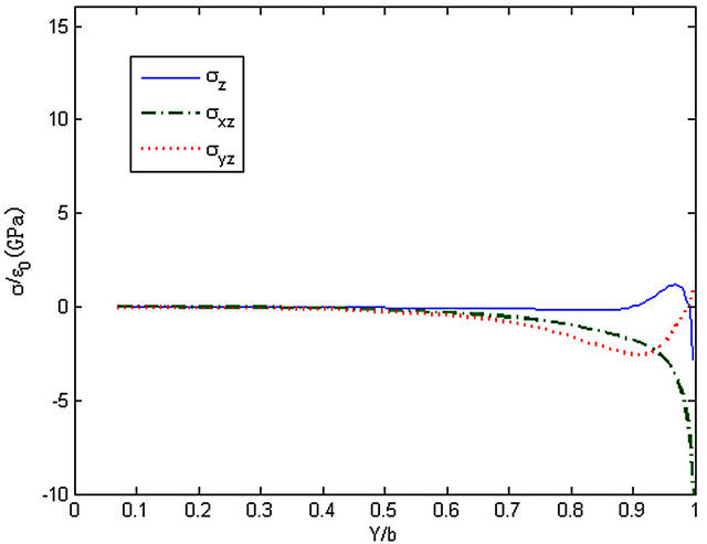
Figure 23. The stresses along y-axis, z = 7h/8.
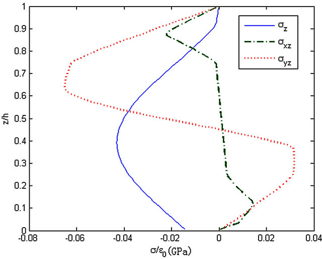
Figure 24. The stresses along z-axis, y = 0.25b.
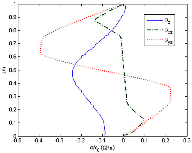
Figure 25. The stresses along z-axis, y = 0.5b.
zero on the surface. And the curves at cross sections y = 0.25b and y = 0.5b are very similar. That stress σz reaches a peak near the interface z = 0.5h. The direction of stress σxz is opposite between the upper and lower half. Furthermore, stress σxz takes turns at the interfaces z = 0.125h, z = 0.25h, z = 0.75h and z = 0.875h. Similar to stress σxz, stress σyz take turns at the interfaces z = 0.25h, z = 0.375h, z = 0.625h and z = 0.75h. And its direction is opposite between the upper and lower half, while it is close to zero at the interfaces z = 0 and z = 0.5h. At the cross section y = 0.99b, stress σz take turns at the interfaces z = 0.125h, z = 0.375h, z = 0.625h and z = 0.875h. It is a tension stress between interfaces z = 0.25h and z = 0.75h while it is a compression in the others. The curve of stress σxz is antisymmetric to the interface z = 0.5h. Moreover, it takes turns at the interfaces z = 0.125h, z = 0.25h, z = 0.75h and z = 0.875h. Similar to stress σxz, the curve of stress σyz is antisymmetric to z = 0.5h and it takes turns at the interfaces except z = 0.5h.
4.4. The Influence of the Ply Angle on the Interlaminar Stresses
The laminated composite plate ([θ/−θ]s) is considered to analyze the influence of the ply angle on the interlaminar stresses. Stress σz along z-axis at the cross section y=0.99b is shown in Figure 27 when the angle is different (θ = 5˚, 15˚, 30˚, 45˚, 60˚, 75˚, 85˚). It can be observed that stress σz is changed with the ply angle apparently while the shapes of the curves in Figure 27 are similar. At z = 0.5h of cross section y = 0.99b, the relationship between the absolute value of stress σz and the ply angle is shown in Figure 28. That when the ply angle ranged between 0˚ and 30˚, the absolute value of stress σz is increased. Moreover, it reaches a maximum as the an gle is equal to 30˚. Then when the ply angle ranged between 30˚ and 60˚, it is decreased with the angle. Besides, it closes to zero when the angle ranged between 60˚ and 90˚.
Stress σxz along z-axis at the cross section y = 0.99b is shown in Figure 29 when the ply angle is different
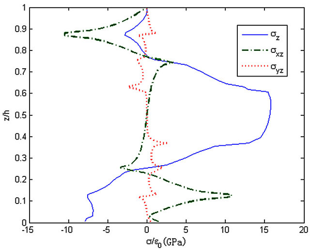
Figure 26. The stresses along z-axis, y = 0.99b.
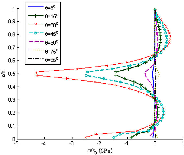
Figure 27. Influence of θ to stress σz along z-axis, y = 0.99b.
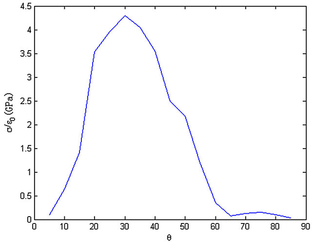
Figure 28. Stress σz changes with θ, y = 0.99b, z = h/2.
(θ = 5˚, 15˚, 30˚, 45˚, 60˚, 75˚, 85˚). Like stress σz, stress σxz is changed with the ply angle apparently while the shapes of the curves in Figure 29 are similar. And at z = 0.5h of cross section y = 0.99b, the relationship between the absolute value of stress σxz and the ply angle is shown in Figure 30. The maximum is happened when the angle is about 20˚, which is different from Figure 28.
Stress σyz along z-axis at the cross section y = 0.99b is shown in Figure 31 when the ply angle is different (θ = 5˚, 15˚, 30˚, 45˚, 60˚, 75˚, 85˚). Like the other two stresses, stress σyz is changed apparently with the ply angle while the shapes of the curves in Figure 31 are similar. And at z = 0.5h of cross section y = 0.99b, the relationship between the absolute value and stress σyz with the ply angle is shown in Figure 32 which is similar to Figure 28.
5. Results and Discussion
The interlaminar stresses are not uniform along y-axis of the laminated composite plate subjected to a uniform axial strain. But it changes sharply in the vicinity of the
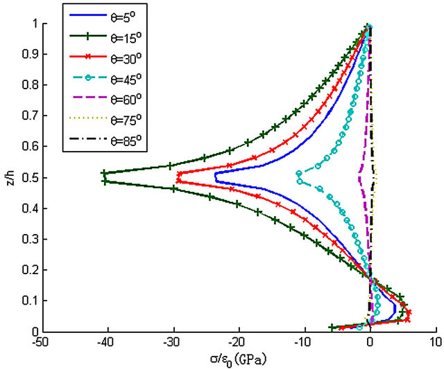
Figure 29. Influence of θ to stress σxz along z-axis, y = 0.99b.
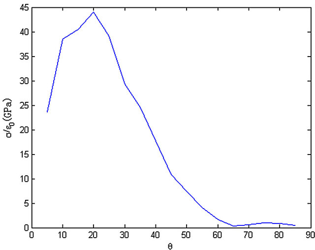
Figure 30. Stress σxz changes with θ, y = 0.99b, z = h/2.
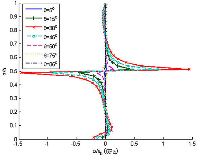
Figure 31. Influence of θ to stress σxz along z-axis, y = 0.99b.
edge and reaches a minimum or maximum at the free edge which makes the delamination phenomenon oc-
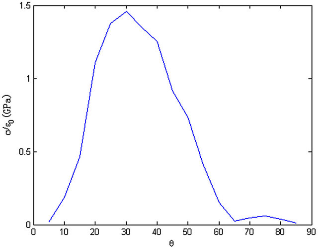
Figure 32. Stress σxz changes with θ, y = 0.99b, z = h/2.
curred to fail the material. In this paper, the interlaminar stresses are calculated for laminated composite plate with different ply manners.
Firstly, the distributions of the interlaminar stresses along y-axis are studied. Stresses σz and σxz change sharply in the vicinity of the free edge, such as increase or decrease sharply or a peak happened near the free edge. Moreover, it reaches a maximum (or minimum) at the edge. Stress σz and σxz are very small in the interior area in comparison with stresses in the vicinity of the free edge. Also stress σyz is very small at the area far from the free edge, but its value is close to zero after a peak happened near the edge, which is different from stresses σz and σxz. In a word, the values of the interlaminar stresses near the free edge are much higher in the interior area. So the failure of material easier happened in the vicinity of free edge than in the interior area.
Secondly, the distributions of the interlaminar stresses along z-axis are studied. The interlaminar stresses are close to zero on the surface. And the stress σyz is very small at the interface z = 0. At the cross section far away from the free edge, stress σz doesn’t change very much and stresses σxz and σyz both take a turn at the interface. In contrary, the interlaminar stresses change very sharply at the vicinity of the free edge. Stresses σz and σxz both reach a peak at the interface while the direction of stress σyz changes to opposite suddenly at the interface ±θ.
At last, the influence of the ply angle on the interlaminar stresses is analyzed for the laminated composite plate ([θ/−θ]s). The values of the interlaminar stresses are changed apparently with the ply angle. But the curves of the stresses along z-axis are similar. The absolute value of the interlaminar stresses is increased as the ply angle ranged between 0˚ and a specific value which is about 20˚ or 30˚, then a decrease process is happened as the ply angle ranged between the specific value and 60˚. Besides, it closes to zero when the angle ranged between 60˚ and 90˚. So when the laminates is angle plied as [θ/−θ]s ,the angle is suggested between 60˚ and 90˚ to lower the free edge effect.
The accuracy can be ensured by using the displacement field presented in this paper. And the validation of using the linear finite element is demonstrated by some numerical results. Also it is convenient that only the linear finite element is used to calculate the interlaminar stresses as the interpolation along z-axis is included in the displacement field. It should be noticed that the finite element used here can be only applied to the laminates subjected to a uniform strain. But it can be easy to be expanded to analyze the other laminates.
6. Acknowledgements
The authors would like to express their gratitude for the support provided by the National Natural Science Foundation of China (NO. 11072151).
REFERENCES
- S. B. Dong, K. S. Pister and R. L. Taylor, “On the Theory of Laminated Anisotropic Shells and Plates,” Journal of the Aeronautical Sciences, Vol. 29, No. 8, 1962, pp. 969- 975.
- E. Reissner and Y. Stavsky, “Bending and Stretching of Certain Types of Heterogeneous Aelotropic Elastic Plates,” Journal of Applied Mechanics, Vol. 28, No. 3, 1961, pp. 402-408. doi:10.1115/1.3641719
- N. J. Pagano, “Stress Fields in Composite Laminates,” International Journal of Solids and Structures, Vol. 14, No. 4, 1978, pp. 385-400. doi:10.1016/0020-7683(78)90020-3
- N. J. Pagano, “Free Dege Stress Fields in Composite Laminates,” International Journal of Solids and Structures, Vol. 14, No. 5, 1978, pp. 401-406. doi:10.1016/0020-7683(78)90021-5
- C.-P. Wu and H.-C. Kuo, “An Interlaminar Stress Mixed Finite Element Method for the Analysis of Thick Laminated Composite Plates,” Composite Structures, vol. 24, No. 1, 1993, pp. 29-42. doi:10.1016/0263-8223(93)90052-R
- H. Matsunaga, “Interlaminar Stress Analysis of Laminated Composite Beams According to Global Higher- Order Deformation Theories,” Composite Structures, Vol. 55, No. 1, 2002, pp. 105-114. doi:10.1016/S0263-8223(01)00134-9
- A. Nosier and A. Bahrami, “Interlaminar Stresses in Antisymmetric Angle-Ply Laminates,” Composite Structures, Vol. 78, No. 1, 2007, pp. 18-33. doi:10.1016/j.compstruct.2005.08.007
- T. S. Plagianakos and D. A. Saravanos, “Higher-Order Layerwise Laminate Theory for the Prediction of Interlaminar Shear Stresses in Thick Composite and Sandwich Composite Plates,” Composite Structures, Vol. 87, No. 1, 2009, pp. 23-35. doi:10.1016/j.compstruct.2007.12.002
- H. S. Kim, S. Y. Rhee and M. Cho, “Simple and Efficient Interlaminar Stresses Analysis of Composite Plates with Internal Ply-Drop,” Composite Structures, vol. 84, No. 1, 2008, pp. 73-86. doi:10.1016/j.compstruct.2007.06.004
- M. Amabili and J. N. Reddy, “A New Non-Linear Higher-Order Shear Deformation Theory Large Amplitude Vibrations of Laminated Doubly Curved Shells,” International Journal of Non-Linear Mechanics, Vol. 45, No. 4, 2010, pp. 409-418. doi:10.1016/j.ijnonlinmec.2009.12.013
- A. K. Miri and A. Nosier, “Interlaminar stresses in Antisymmetric Angle-Ply Cylindrical Shell Panels,” Composite Structures, Vol. 93, No. 2, 2011, pp. 419-429. doi:10.1016/j.compstruct.2010.08.038
- X. H. Ren, W. J. Chen and Z. Wu, “A New Zig-Zag Theory and C0 Bending Element for Composite and Sandwich Plates,” Archive of Applied Mechanics, Vol. 81, No. 2, 2011, pp. 185-197. doi:10.1007/s00419-009-0404-0
- J. L. Mantari, A. S. Oktem and C. Guedes Soares, “A New Higher Order Shear Deformation Theory for Sandwich and composite Laminated Plates,” Composites Part B: Engineering, Vol. 43, No. 3, 2012, pp. 1489-1499.
- A. Nosier and M. Maleki, “Free-Edge Stresses in General Composite Plates,” International Journal of Mechanical Sciences, vol. 50. No. 10-11, 2008, pp. 1435-1447. doi:10.1016/j.ijmecsci.2008.09.002
- C.-F. Liu and H.-S. Jou, “A New Finite Element Formulation for Interlaminar Stress Analysis,” Computer and Structures, Vol. 48. No. 1, 1993, pp. 135-139. doi:10.1016/0045-7949(93)90464-O
Appendix
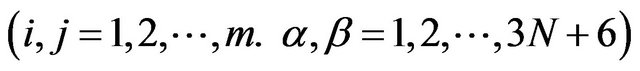
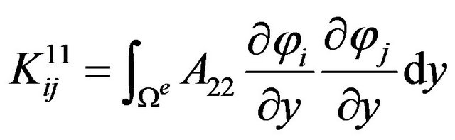
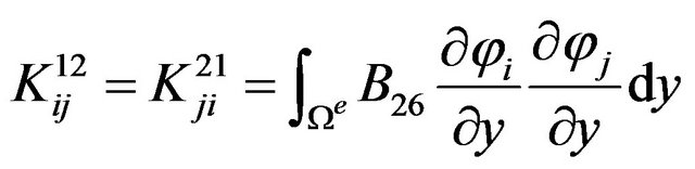
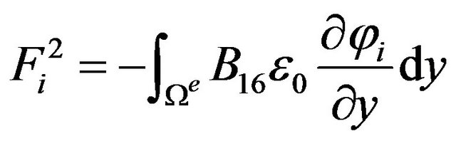
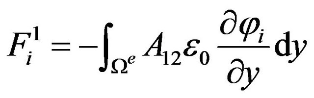
The definite expression of the finite element equation Kd = F can be written as below:
where . m is the number of the node of the element. N is the number of the numerical layers along z-axis. The expressions of
 ![]() and
and 
 can be written as below:
 ,
,
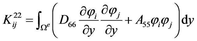
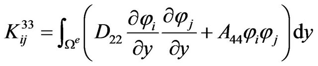
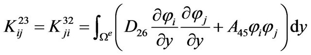

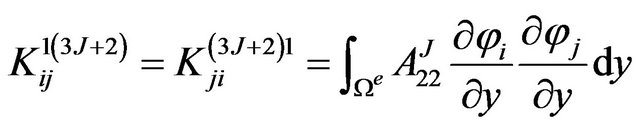
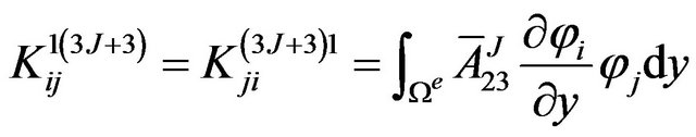
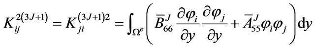


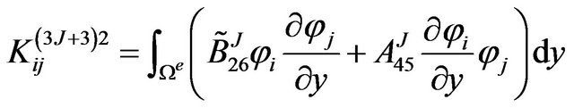

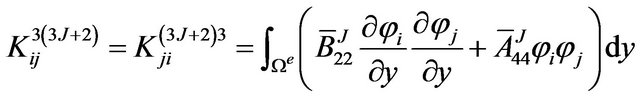
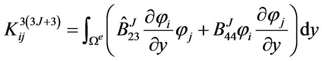
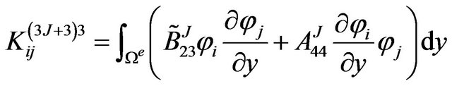
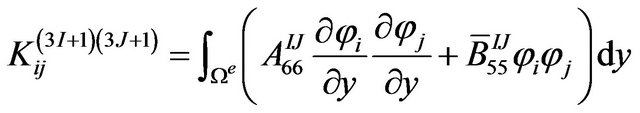
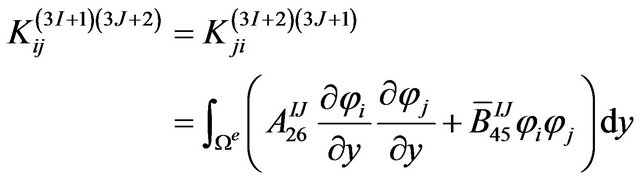
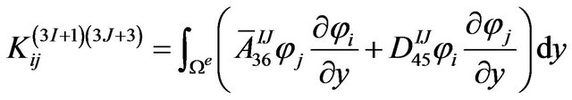
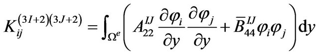
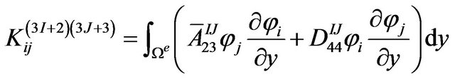
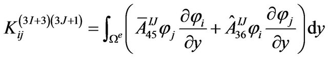
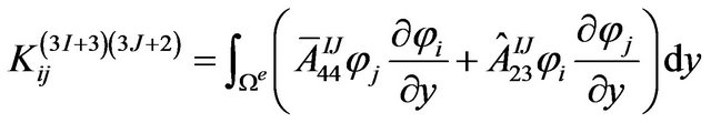
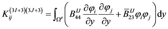

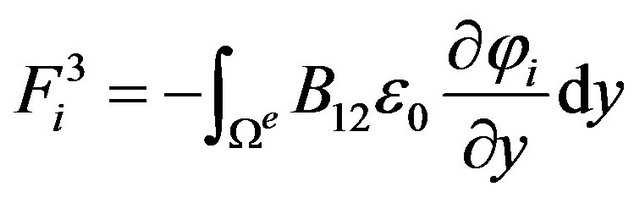
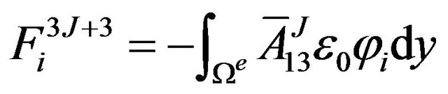
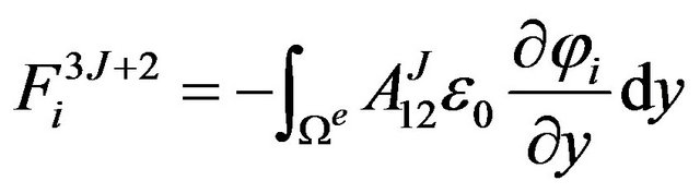
where, .
.  and
and  are the interpolation shape function of the node.
  is the uniform axial strain along x-axis. And the coefficient expressions in
 ![]() and
and  can be written as:
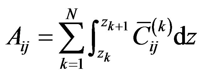
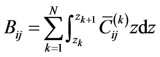
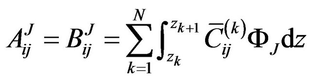
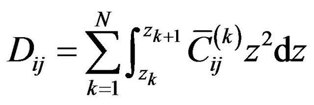
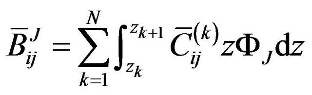
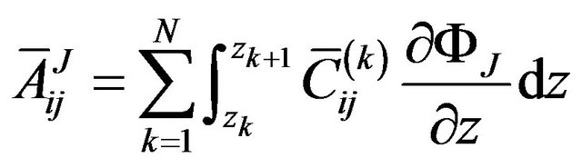
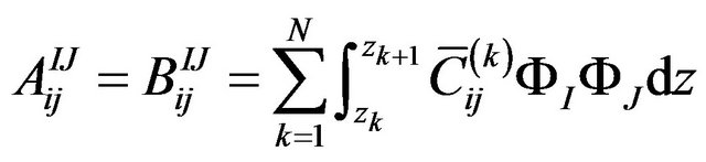
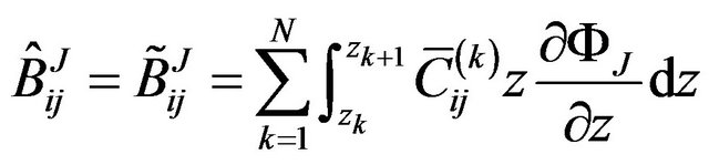
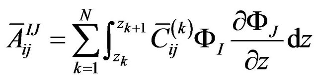
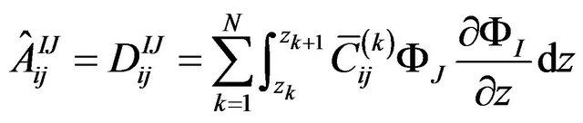
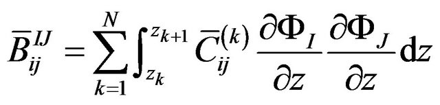
where, z is the coordinate of z-axis. zk is z-coordinate of the upper surface of the kth layer while zk+1 is z-coordinate of the lower surface of the kth layer.  is the offaxis stiffness coefficient of the kth layer (i, j = 1, 2, 3, 4, 5, 6).
  and
and  are the interpolation function of the Equations (1) and (2).