Journal of Geoscience and Environment Protection
Vol.07 No.04(2019), Article ID:91670,17 pages
10.4236/gep.2019.74001
The Application of the Generalized Finite Difference Method (GFDM) for Modelling Geophysical Test
Angel Muelas1, Eduardo Salete1, Juan José Benito1, Francisco Ureña2, Luis Gavete3, Miguel Ureña1
1UNED, ETS Ingenieros Industriales, C/Juan del Rosal, Madrid, Spain
2UCLM, IMACI, Ciudad Real, Spain
3UPM, ETSIM, Madrid, Spain

Copyright © 2019 by author(s) and Scientific Research Publishing Inc.
This work is licensed under the Creative Commons Attribution International License (CC BY 4.0).
http://creativecommons.org/licenses/by/4.0/


Received: February 20, 2019; Accepted: April 7, 2019; Published: April 10, 2019
ABSTRACT
The possibility of using a nodal method allowing irregular distribution of nodes in a natural way is one of the main advantages of the generalized finite difference method (GFDM) with regard to the classical finite difference method. Moreover, this feature has made it one of the most-promising meshless methods because it also allows us to reduce the time-consuming task of mesh generation and the numerical solution of integrals. This characteristic allows us to shape geological features easily whilst maintaining accuracy in the results, which can be a source of great interest when dealing with this kind of problems. Two widespread geophysical investigation methods in civil engineering are the cross-hole method and the seismic refraction method. This paper shows the use of the GFDM to model the aforementioned geophysical investigation tests showing precision in the obtained results when comparing them with experimental data.
Keywords:
Meshless Methods, Generalized Finite Difference Method, Geophysics

1. Introduction
Geotechnical geophysical tools are routinely used to image the subsurface of the Earth and determine site geology, stratigraphy, and rock quality. Commonly employed geophysical investigation methods include seismic refraction, seismic reflection, MASW, cross-hole seismic tomography, electrical resistivity, GPR (Ground Penetrating Radar), electromagnetics, gravity, etc.
The cross-hole seismic technique determines the compressional (P-) and/or shear (S-) wave velocity of materials at different depths. Cross-hole testing takes advantage of generating and recording (seismic) body waves, both the P-waves and S-waves, at selected depth intervals where the source and receiver(s) are maintained at equal elevations for each measurement.
P-waves are generated with a sparker or small explosive device such that along the assumed straight-ray propagation path the seismic impulse compresses and rarefies the materials radially toward the receiver borehole(s). S-waves generated in cross-hole testing may be split into two wave types, each with different particle motions―SV- and SH-waves, respectively.
The seismic refraction method is used to estimate depths and seismic velocities of geological layers. Seismic velocities can assist in the interpretation of the geological profile as well as the evaluation of the rippability of bedrock.
In the seismic refraction method, a seismic source (a hammer hitting on a plate, an explosive, etc.) is used to generate body waves, most commonly, P-waves.
The wave arrival time is measured by a series of evenly spaced geophones located on the ground surface.
The seismic waves propagate downwards through the ground until they are reflected or refracted off subsurface layers. Refracted waves are detected by arrays of a number of geophones spaced at regular intervals of 1 - 10 meters, depending on the desired depth penetration of the survey.
Some head waves enter a high velocity medium near the critical angle and travel in the high velocity medium nearly parallel to the interface between layers. Then, the wave refracted along that interface will overtake the direct wave at some distance from the source. This point at which the refracted wave overtakes the direct wave arrival is known as the critical distance and is used to estimate the depth to the refracting surface.
The GFDM has been proven to be a successful method to model seismic wave propagation using regular or irregular meshes. Researchers as Jensen (1972) , Liszka and Orkisz (1980) , Orkisz (1998) and Perrone and Kao (1975) have contributed to developing the GFDM in different aspects of its applications. Benito, Gavete, & Ureña (2001) have developed the explicit formulae and have also applied this meshless method to solve the advection diffusion equation (Ureña, Benito, & Gavete, 2011) to solve parabolic and hyperbolic equations (Benito, Ureña, & Gavete, 2007) and to solve second order non-linear elliptic partial differential equations (Gavete et al., 2017) .
The application of GFDM to the solution of the problem of seismic wave propagation was introduced by Benito et al. (2017) where a GFD scheme for elastic, homogeneous isotropic medium was proposed and the stability and dispersion studied. A perfectly matched layer (PML) absorbing boundary was included in the numerical model by Benito et al. (2013) , its stability was analyzed in (Salete et al., 2017) and the influence of the topography and domain irregularities was shown in (Benito et al., 2015) . An adaptive process to minimize the influence of the irregularity of the star nodes distribution on the dispersion was proposed in (Salete et al., 2011) . New schemes for seismic wave propagation in Kelvin-Voight viscoelastic media and some improvements in the heterogeneous schemes to deal with irregular interfaces were proposed in (Benito et al., 2013) , (Benito et al., 2018) .
Moreover, the application of the finite-difference method to the seismic wave propagation and earthquake problems has been also tackled by authors as Boore, Levander, Carcione and Moczo (1998) among others.
In this paper, the GFDM has been applied to model two widespread geophysical tests, namely the cross-hole method and the Seismic refraction method trying to analyze the possibility of using it in other geophysical problems.
The paper is organized as follows. In Section 2 the formulation of GFDM to solve seismic wave propagation problem containing the stability condition and the scheme in PML has been included. The geophysical investigation modelling is shown in Section 3 and the obtained results are analyzed and evaluated in Section 4. Finally, in Section 5, some conclusions are obtained.
2. Fundamentals of the GFDM
2.1. Explicit Formulae
Let be a domain and
a discretization of the domain Ω with N points. Each point of the discretization M is denoted as a node.
For each one of the nodes of the domain, where the value of U is unknown, Es-star is defined as a set of selected points with the central node x0 Î M and is a set of points located in the neighborhood of x0. In order to select the points, different criteria as the four quadrants or distance can be used (Benito et al., 2001) .
We consider an Es-star with the central node x0, where (x0, y0) are the coordinates of the central node, (xi, yi) are the coordinates of the ith node in the Es-star, and hi = xi − x0 and ki = yi − y0. If U0 = U(x0) is the value of the function at the central node of the star and Ui = U(xi) are the function values at the rest of the nodes, with , then, according to the Taylor series expansion it is known that:
(1)
If in Equation (1) the higher than second order terms are ignored, a second order approximation for the Ui function is obtained. This is indicated as ui. It is then possible to define the function B(u) as:
(2)
where are positive symmetrical weighting functions, having the property as defined in Lancaster and Salkauskas (1986) that are functions decreasing monotonically in magnitude as the distance to the center of the weighting function increases. See also Levin (1998) for more detail.
Some weighting functions as potential or exponential can be
used (Benito et al., 2001) , where . If the norm given by Equation (2) is minimized with respect to the partial derivatives, the following system of linear equations is obtained (for each node of the discretization)
(3)
The matrix A is a positive definite matrix and the approximation is of second order, (Gavete et al., 2017) .
The solution of system Equation (3) is unique and it is a linear combination of the function values obtained at the nodes. Then
(4)
with
(5)
The explicit expressions of matrices A, D, b and coefficients m0, mi may be seen in (Benito et al., 2001; Benito et al., 2015; Benito et al., 2007) .
2.2. Equation of Motion, Boundary Conditions and PML
The equations of motion for a perfectly elastic, homogeneous and isotropic medium in the domain are
(6)
The Ui are the components of the displacements, ρ is the density and λ and µ are Lame’s elastic coefficients.
In this paper two types of boundary conditions are considered: Dirichlet boundary conditions and free surface. On the free surface, the following conditions we impose
(7)
where gi(t) is equal to zero when there are not forces on the surface.
PML x-dir can be conceptually assumed up by a single transformation of the original equation. Then, wherever and x derivative appears in the wave equations, it is replaced in the form
(8)
where in Equation (8).
Substituting the expression Equation (8) in Equation (6) the equations for PML part (Benito et al., 2013) , are:
(9)
2.3. Explicit Generalized Differences
The explicit scheme formulae for the second spatial derivatives with second order approximation (see Equation (4)), are
(10)
where hl = xl − x0 and kl = yl − y0 the superscript n denotes time step, the superscripts 0 and l refer to the central node and the rest of nodes of the star respectively and s is the number of nodes in the star (in this work s = 8 and the star nodes are selected by using the distance criteria) (Benito et al., 2001) .
are the coefficients that multiply the approximate values of the functions Ui at the central node ( ) for the time n∆t in the generalized finite difference explicit expressions for the space derivatives, and are the coefficients that multiply the approximate values of the functions Ui at the other nodes of the star ( ). In all these expressions the cross-terms are equal.
The replacement in Equation (1) of the explicit expressions obtained for the spatial derivatives (Equation (10)) and the central-difference formula for the time derivative lead to the explicit differences scheme:
(11)
and the scheme in GFDM for the PML part can be obtained in a similar way:
(12)
where
In order to implement the free surface conditions, Equation (7), we need to add the same number of nodes outside of our domain as there exists on the free boundary and place them near it. Substituting the first order derivatives that appear in the free surface conditions Equation (7) by the explicit expressions (Equation (10)) the system of 2p equations is obtained:
(13)
where the 2p unknowns are the displacements in the p added nodes. These unknowns appear in the summation.
2.4. Stability of the GFD Scheme and Stability of PML Regions
The stability of the schemes has already been studied in (Ureña et al., 2011) and its formulation leads to
(14)
where α and β are the velocities of the P-waves and S-waves respectively.
The stability analysis in the continuum of the PML has already been studied in (Salete et al., 2011) .
The dispersion for the phase and group velocities have also been studied in depth in (Gavete et al., 2017) .
2.5. Heterogeneous Formulation
If the density and Lamé coefficients λ and µ are functions of spatial variables, in agreement with Moczo (1998) , in seismological problems the heterogeneous approach can be complicated and, then, so-called heterogeneous formulation is preferred. Therefore, the same formulae are used for all points in the domain and material discontinuities are accounted for spatial variation of the material parameters (Benito et al., 2013) .
3. Geophysical Investigation Modelling
The following is the application of the GFDM to model of a cross-hole and model of seismic refraction studies of the aforementioned seismic tests.
3.1. Model of a Cross-Hole Test
A geotechnical investigation has been carried out to elaborate a geotechnical profile on a construction site. Three boreholes with core recovery and an additional cross-hole test were performed in order to obtain a seismic velocity vs. depth profile. Based on the geotechnical investigation aforementioned, the subsoil comprises an upper layer of medium dense to dense sand up to 6-meter depth, overlying a very dense silty sand layer. The λ parameter, the dynamic Shear Modulus and the compression and shear wave velocity vs. depth are shown in Figure 1.
The dynamic parameters shown in Figure 1 have been assigned to the subsoil as a function of soil depth.
The cross-hole test has been analyzed by in a GFDM model, applying a vertical pulse (to generate S-waves) and a horizontal pulse (to generate P-waves) at different depths. The step pulse is applied for a time increment of t = 1e−5 sec. The model is 16 m (vertical) × 6 m (horizontal), with a regular node spacing of 0.05 m. The number of nodes is 38,400. The star is made up of eight nodes plus the central node. The selection of nodes associated to each central node is based


Figure 1. Dynamic soil properties (Borehole CH03).
on the distance criterion. The weighting function adopted is the potential function 1/(dist)3. A free surface boundary condition has been imposed to the upper and right limits of the model. An absorbing boundary condition (Perfectly Matched Layer) has been imposed to the lower and left limits of the model.
Figure 2 shows the moment at which the front S-wave reaches the geophone located at 9-meter depth in the GFDM model. The shear, head or Von-Schmidt and surface or Rayleigh waves can clearly be seen in Figure 2.
The vertical displacement over time for the geophone located at 9-meter depth is shown in Figure 3. The shear wave velocity is obtained from the time of wave arrival, taking into account the distance between the source and the geophone (3 meters).
By applying a horizontal pulse at the source location, the P-waves propagation has also been analyzed. The pressure or dilatational, shear, head and surface waves can be seen in Figure 4.
The curve that appears in Figure 5 shows the horizontal displacement ux over time for the geophone located at 9-meter depth. The P-waves velocity is obtained from the time of wave arrival, similarly to the S-waves case.
3.2. Model of Seismic Refraction
The seismic refraction method is usually performed in quarries or open-pit mines to make an estimate of the rock volume that may be extracted from the site and the most appropriate excavation method. For example, the seismic refraction method carried out in a quarry in Valparaiso (Chile) to quantify the weathered and fresh rock volume. The layout of the seismic refraction profiles is shown in Figure 6. As a result of the geophysical study, the longitudinal profile shown in (Figure 7) was obtained.
Basically, the subsoil is composed of three layers (sandy oil, weathered rock and fresh rock).
The purpose of the model is to simulate the real geophysical investigation, measuring the travel time for the wave to reach the geophones located on the

Figure 2. Cross-hole test model-front shear waves reaching the 9-meter depth geophone.
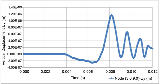
Figure 3. Vertical displacement vs. time for geophone located at 9 m depth.
ground surface along the profile. The real data obtained from the geophysical investigation are shown in Figure 8. The different dromochrones (distance vs. travel time curves) have been drawn for the different pulse locations. Three slopes may be distinguished in most of these curves, corresponding to the three soil layers aforementioned: sandy soil, weathered rock and fresh rock. Three representative dromochrones have been selected (Figure 9) to enhance these three slopes.
The slope of the first section of the three curves is very similar, leading to a seismic velocity of 350 - 500 m/s for the sandy soil layer. Nevertheless, the point where the curve changes its slope depends on the thickness of the soil layer. On curve 2, the time when the refracted wave reaches the direct wave is shorter than the one for curves 1 and 3. This difference leads to a smaller thickness of layer 1 in the neighborhood of x = 30 m. Regarding the second section of the curves, the
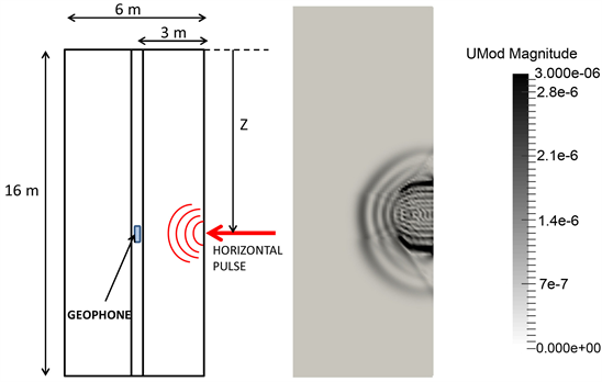
Figure 4. Front p-waves reaching the 9 m depth geophone.

Figure 5. Horizontal displacement vs. time for geophone located at 9 m depth.

Figure 6. Seismic refraction profiles layout.
seismic velocity obtained for the weathered rock layer ranges from 1000 to 2000 m/s. Finally, the seismic velocity for the third layer (fresh rock) ranges from 5000 to 11,000 m/s.

Figure 7. Geological profile.

Figure 8. Geophysical investigation data: Dromochrones for different pulse locations.
A GFDM model has been used to model the seismic refraction investigation (Figure 10). The horizontal and vertical dimensions of the model are 200 meters and 60 meters, respectively. A regular mesh of nodes has been adopted with a node spacing of 1 meter, leading to a total number of nodes of 12,000. Every star

Figure 9. Representative travel time vs. distance curves.

Figure 10. Subsoil model to analyze the seismic refraction method.
is made up of eight nodes plus the central node. The selection of nodes associated to each central node is based on the distance criterion. The weighting function adopted is the potential function 1/(dist)3. A free surface boundary condition has been imposed to the upper limit of the model. An absorbing boundary condition (Perfectly Matched Layer) has been imposed to the lower and side limits of the model. The vertical pulse applied at the surface at x = 50 m. (50 meters from the left border) corresponds to the central lobe of a Ricker wavelet. The parameters for the Ricker wavelet adopted are the following ones: Ricker wavelet:
where: ts = 0.00015 s and fM = 1418 s−1.
The time increment adopted is t = 0.00005s. Therefore, the central lobe for the Ricker wavelet can be defined by 7 points, from t = 0 s. until t = 0.0003 s.
The main goal of the model is to reproduce the distance vs. travel time curves obtained in the geophysical investigation. The curves depend not only on the elastic parameters of the soil layers (Youngs Modulus, Shear Modulus), but on their thickness. By varying the elastic parameters and the thickness of the soil layers, a distance vs. travel time curve has been obtained whose seismic velocities lie within the real velocities range. Figure 11 shows the dromochrone obtained from the model.
The seismic velocities calculated from the model data curve in Figure 11 are the following ones:
Layer 1 (sandy soil): vp = 460 m/s.
Layer 2 (weathered rock): vp = 1590 m/s.
Layer 3 (fresh rock): vp = 5000 m/s.
In Figure 12 three curves showing the wave amplitude vs. time are shown. The red one corresponds to the point A (50.0, 0.0) where the pulse has been applied. The green one corresponds to the node B (50.0, 7.0), located 7 meters below the pulse node; and the blue one shows the curve for node C (50.0, 9.0), located 9 meters below the pulse node, that is, 1 meter in the second soil layer (weathered rock).
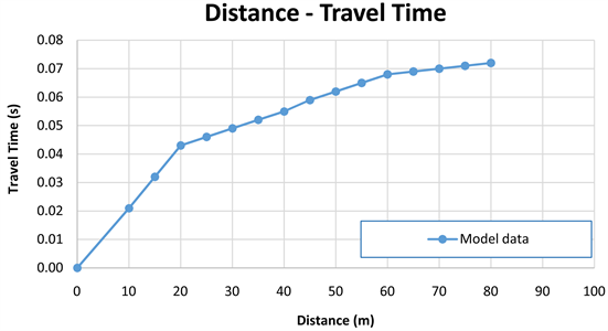
Figure 11. Distance vs. travel time curves from model.

Figure 12. Wave amplitude vs. time curves for nodes A (50.0, 0.0), B (50.0, 7.0), and C (50.0, 9.0).
To illustrate the capability of the model to reproduce the refraction of waves, several screenshots of the model have been shown in Figures 13-15. The refraction is clearly modelled between layers 1 and 2, and between layers 2 and 3.
The graphic scale has been adjusted to enhance the wavefront, which results in a higher color saturation for the zones with higher amplitude. The P waves wavefront has been indicated in the figures, showing the higher wave velocity in the layer 2 compared to layer 1. Besides, the Rayleigh waves can be identified at the surface close to the point where the pulse has been applied. In addition, the refracted waves wavefront reaching the surface can be clearly distinguished in Figure 15.

Figure 13. P-waves wavefront in layers 1 and 2.
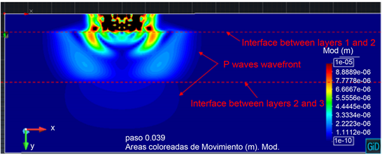
Figure 14. P-waves wavefront in layers 2 and 3.

Figure 15. Refracted waves reaching the surface.
4. Discussion
In this chapter the results of the modelling are analyzed and evaluated.
4.1. Model of a Cross-Hole Test
Figure 16 shows the comparison between the actual seismic velocities recorded in the cross-hole test and those obtained with the model.
As it may be observed in Figure 16, the model-calculated seismic velocities match satisfactorily to those obtained in the cross-hole test, with a 5% maximum deviation. It is therefore concluded that the model is capable to reproduce accurately a cross-hole test, with minimum error in P-wave and S-wave velocities.
4.2. Model of Seismic Refraction
Figure 17 shows the real dromochrones along with that one obtained from the model.
The seismic velocities calculated from the GFDM fall within the range for the seismic velocities derived from the field investigation. Therefore, it can be concluded that the GFDM model may successfully simulate the real seismic refraction investigation to obtain the thicknesses and the seismic velocities of the different layers of a geological profile.
It is also necessary to clarify that the discretization of a geological profile in a finite number of different layers is a simplified view of the geology. Frequently, the edge between two layers is not a well-defined line, but a zone where the transition from one layer to another takes place. It happens, for example, in the transition from weathered and fresh rock. This explains the abrupt change in the
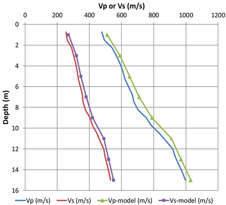
Figure 16. Comparison between actual and model-obtained seismic velocities.
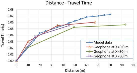
Figure 17. Distance vs. travel time curves from model and real geophysical investigation.
slope of the obtained curves, characteristic of these kinds of simulations.
5. Conclusion
This paper describes the fundamentals of the GFDM, which has been proven to be a successful method to model seismic wave propagation using regular or irregular meshes.
It has been shown the use of the GFDM to model two of the most widespread geophysical investigation methods used in civil engineering: Cross-hole method and the Seismic Refraction method with the intention of analyzing its effectiveness in order to deal with other kinds of geophysical problems.
It has been concluded that a GFDM model is capable to reproduce accurately a cross-hole test. The model-calculated seismic velocities match satisfactorily to those obtained in the cross-hole test, with a 5% maximum deviation.
In addition, this paper shows the use of the GFDM to model accurately the seismic refraction method, obtaining similar seismic velocities to the ones derived from the real data obtained from the geophysical investigation.
The obtained results can lead to the use of GFDM to solve many geophysical problems due to the features of this method, and the possibility of using irregular meshes can be profitable. Moreover, our research group has obtained new schemes for seismic wave propagation in Kelving-Voight viscoelastic media (Benito et al., 2018) and also improvements in the heterogeneous schemes to deal with irregular interfaces (Benito et al., 2013, 2018) . These new possibilities together with the good results obtained in the geophysical test presented here, expand the limits of possible applications of GFDM in this field to problems like modelling of geologic discontinuities (faults, fractures…), karstic cavities, anisotropic rock masses, soil-structure interaction problems, earthquake ground motion amplification, etc.
Acknowledgements
The authors acknowledge the support of the Escuela Técnica Superior de Ingenieros Industriales (UNED) of Spain, project 2019-IFC02, and of the Universidad Politécnica de Madrid (UPM) (Research groups 2019).
Conflicts of Interest
The authors declare no conflicts of interest regarding the publication of this paper.
Cite this paper
Muelas, A., Salete, E., Benito, J. J., Ureña, F., Gavete, L., & Ureña, M. (2019). The Application of the Generalized Finite Difference Method (GFDM) for Modelling Geophysical Test. Journal of Geoscience and Environment Protection, 7, 1-17. https://doi.org/10.4236/gep.2019.74001
References
- 1. Benito, J. J., Ureña, F., & Gavete, L. (2001). Influence Several Factors in the Generalized Finite Difference Method. Applied Mathematical Modeling, 25, 1039-1053. https://doi.org/10.1016/S0307-904X(01)00029-4 [Paper reference 5]
- 2. Benito, J. J., Ureña, F., & Gavete, L. (2007). Solving Parabolic and Hyperbolic Equations by the Generalized Finite Difference Method. Journal of Computational and Applied Mathematics, 209, 208-233. https://doi.org/10.1016/j.cam.2006.10.090 [Paper reference 2]
- 3. Benito, J. J., Ureña, F., Gavete, L., Salete, E., & Muelas, A. (2013). A GFDM with PML for Seismic Wave Equations in Heterogeneous Media. Journal of Computational and Applied Mathematics, 252, 40-51. https://doi.org/10.1016/j.cam.2012.08.007 [Paper reference 5]
- 4. Benito, J. J., Ureña, F., Gavete, L., Salete, E., & Ureña, M. (2017). Implementations with Generalized Finite Differences of the Displacements and Velocity-Stress Formulation of Seismic Wave Propagation Problem. Applied Mathematical Modelling, 52, 1-14. https://doi.org/10.1016/j.apm.2017.07.017 [Paper reference 1]
- 5. Benito, J. J., Ureña, F., Salete, E., Muelas, A., Gavete, L., & Galindo, R. (2015). Wave Propagation in Soils Problems Using the Generalized Finite Difference Method. Soil Dynamics and Earthquake Engineering, 79, 190-198. https://doi.org/10.1016/j.soildyn.2015.09.012 [Paper reference 2]
- 6. Benito, J. J., Ureña, F., Ureña, M., Salete, E., & Gavete, L. (2018). Schemes in Generalized Finite Differences for Seismic Wave Propagation in Kelvin-Voight Viscoelastic Media. Engineering Analysis with Boundary Elements, 95, 25-32. https://doi.org/10.1016/j.enganabound.2018.06.017 [Paper reference 2]
- 7. Benito, J. J., Ureña, F., Ureña, M., Salete, E., & Gavete, L. (2018). A New Meshless Approach to Deal with Interfaces in Seismic Problems. Applied Mathematical Modelling, 58, 447-458. https://doi.org/10.1016/j.apm.2018.02.014
- 8. Gavete, L., Ureña, F., Benito, J. J., Garcia, A., Ureña, M., & Salete, E. (2017). Solving SECOND Order Non-Linear Elliptic Partial Differential Equations Using Generalized Finite Difference Method. Journal of Computational and Applied Mathematics, 318, 378-387. https://doi.org/10.1016/j.cam.2016.07.025 [Paper reference 3]
- 9. Jensen, P. S. (1972). Finite Difference Technique for Variable Grids. Computer& Structures, 2, 17-29. https://doi.org/10.1016/0045-7949(72)90020-X [Paper reference 1]
- 10. Lancaster, P., & Salkauskas, K. (1986). Curve and Surface Fitting. Cambridge, MA: Academic Press. [Paper reference 1]
- 11. Levin, D. (1998). The Approximation Power of Moving Least Squares. Mathematics of Computation, 67, 1517-1531. https://doi.org/10.1090/S0025-5718-98-00974-0 [Paper reference 1]
- 12. Liszka, T., & Orkisz, J. (1980). The Finite Difference Method at Arbitrary Irregular Grids and Its Application in Applied Mechanics. Computer & Structures, 11, 83-95. https://doi.org/10.1016/0045-7949(80)90149-2 [Paper reference 1]
- 13. Moczo, P. (1998). Introduction to Modelling Seismic Wave Propagation by Finite Difference Method, Lectures Notes, Kyoto. [Paper reference 2]
- 14. Orkisz, J. (1998). Finite Difference Method. In M. Kleiber (Ed.), Handbook of Computational Solid Mechanics (Part III). Berlin: Spriger-Verlag. [Paper reference 1]
- 15. Perrone, N., & Kao, R. (1975). A General Finite Difference Method for Arbitrary Meshes, Computer& Structures, 5, 45-58. [Paper reference 1]
- 16. Salete, E., Benito, J. J., Ureña, F., Gavete, L., Ureña, M., & Garcia, A. (2017). Stability of Perfectly Matched Layer Regions in Generalized Finite Difference Method for Wave Problems. Journal of Computational and Applied Mathematics, 312, 231-239. https://doi.org/10.1016/j.cam.2016.05.027 [Paper reference 1]
- 17. Salete, E., Ureña, F., Gavete, L., & Benito, J. J. (2011). A Note in the Application of the Generalized Finite Difference Method to Seismic Wave Propagation in 2-D. Journal of Computational and Applied Mathematics, 236, 3016-3025. [Paper reference 2]
- 18. Ureña, F., Benito, J. J., & Gavete, L. (2011). Application of the Generalized Finite Difference Method to Solve the Advection-Diffusion Equation. Journal of Computational and Applied Mathematics, 235, 1849-1855. https://doi.org/10.1016/j.cam.2010.05.026 [Paper reference 1]