Modern Mechanical Engineering
Vol. 3 No. 2A (2013) , Article ID: 33472 , 10 pages DOI:10.4236/mme.2013.32A001
Artificial Neural Networks for Controlling the Temperature of Internally Cooled Turning Tools
1UPM Ltd., Swindon, England
2Brunel University, London, England
3Technische Universität, Berlin, Germany
Email: fpwardle@upm.org.uk
Copyright © 2013 Frank Wardle et al. This is an open access article distributed under the Creative Commons Attribution License, which permits unrestricted use, distribution, and reproduction in any medium, provided the original work is properly cited.
Received March 21, 2013; revised April 27, 2013; accepted May 19, 2013
Keywords: Control Systems; In-Process Control; Artificial Neural Network; Machine Tools
ABSTRACT
By eliminating the need for externally applied coolant, internally cooled turning tools offer potential health, safety and cost benefits in many types of machining operation. As coolant flow is completely controlled, tool temperature measurement becomes a practical proposition and can be used to find and maintain the optimum machining conditions. This also requires an intelligent control system in the sense that it must be adaptable to different tool designs, work piece materials and machining conditions. In this paper, artificial neural networks (ANN) are assessed for their suitability to perform such a control function. Experimental data for both conventional tools used for dry machining and internally cooled tools is obtained and used to optimise the design of an ANN. A key finding is that both experimental scatter characteristic of turning and the range of machining conditions for which ANN control is required have a large effect on the optimum ANN design and the amount of data needed for its training. In this investigation, predictions of tool temperature with an optimised ANN were found to be within 5˚C of measured values for operating temperatures of up to 258˚C. It is therefore concluded that ANN’s are a viable option for in-process control of turning processes using internally controlled tools.
1. Introduction
A closed loop cooling system integrated with a novel design of tool insert, Figure 1, has many advantages: it eliminates a potential health hazard for machine operators; it is environmentally friendly as there is no coolant wastage; it consumes less power; swarf is easier to dispose of and it has the potential to reduce machine operating costs, [1]. However, confining coolant to internal channels built into the tool insert, presents new challenges: first of all, it will inevitably change the way in which the heat produced by the cutting operation is distributed and disposed of and secondly it will change the state of lubrication at the tool—work interface. This paper is concerned with the first of these challenges where, with the new technology, there is a risk that the local temperature at the cutting edge of the tool, may, under some machining conditions, exceed a permissible threshold and therefore reduce or at least offset any benefit in tool life.
As for internally cooled tools, coolant is completely under control, the measurement of tool temperature becomes a more meaningful and practical proposition. It is not subject to large fluctuations by small adjustments of coolant flow and direction as is the case for externally applied coolant and it therefore relates, to a much greater extent, to the machining conditions, work piece material, tool design and state of wear. Thus, routinely monitoring the temperature of internally cooled tools is one way of observing and hence avoiding the conditions that may create excessively high temperatures. Furthermore, there is now a wealth of evidence to show [2,3] that for many materials there is an optimum cutting temperature which gives maximum tool life and good surface integrity so to be able to control tool temperature has real practical advantages. However this requires tool temperature measurement to be combined with an intelligent control system that can interpret the measurements and signify some form of corrective action. For example, simply knowing temperature allows a judgment to be made about
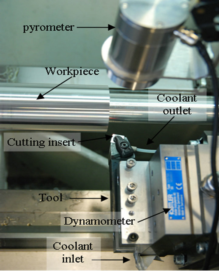
Figure 1. Experimental apparatus.
whether it is too high for the tool or work piece material, however knowing the machining conditions along with the temperature also enables the state of tool wear to be assessed when the temperature is well within material limits. Control systems based on artificial neural networks (ANN) are well suited to this form of decision making. They need to be trained with experimental data to generate a structured relationship between a number of input variables, in this case, machining conditions and an output variable-tool temperature. This relationship provides a reference for interpreting any new tool temperature measurements taken for any machining conditions within an allowable range. Furthermore, the ANN may be retrained any number of times enabling the interpretation tool temperature to be adapted to different work piece materials and tool designs.
Evaluating the benefit of using an ANN based system for controlling the temperature of internally cooled turning tools is the main objective of this paper. In this work, the tool is part of a system that incorporates a variable speed coolant delivery pump so that for a given tool design and work piece material the dominant input variables are coolant flow rate, cutting speed, cutting depth and feed/rev. Essential to the use of an ANN for controlling tool temperature in this system is how accurately it can predict tool temperature given these four input variables. But also of importance is how the prediction accuracy depends on the amount of experimental data and the time required for training.
Past work on ANN’s applied to process/machine control is extensive with more than 1000 papers published since 1990. Whilst there are many types of ANN that can be used for machine tool or industrial process control those based on the Multi Layer Perceptron (MLP) have been used in more than 60% of investigations and have met with most success, [4]. They have generally employed an activation function attached to hidden neurons to improve the accuracy of prediction for the continuous and nonlinear target data characteristic of real control systems. Training has generally been performed off line utilizing back propagation or feed forward algorithms i.e. [5-14]. However what isn’t clear from the published work is a strategy for determining the optimum ANN design for a given application. ANN designs vary widely and in many publications there is no indication as to how a particular design has been arrived at whilst in others, trial and error techniques or systematic variation of parameters have been used to determine an optimum design based on application specific, experimental data. Even in publications where systematic optimization of the ANN design has been undertaken, there have been apparently contradictory findings. For example, [15] found the best results were obtained with a low number of neurons in the hidden layer whilst [16] concluded that increasing the number of neurons improved the results. Alternatively [6] concluded that best results were achieved with an optimum number of neurons. Ref [17] presents the results of a wide ranging investigation into the effect of ANN design on prediction accuracy for data associated with wound toroidal cores. In this case, accuracy improved with the total number of neurons in the hidden layers but it didn’t matter whether they were arranged in a single layer or several layers.
The lack of clear guide lines for ANN design and apparently contradictory findings of past work, at least in relation to process control, suggests ANN design and hence performance is strongly dependent on the experimental data it is required to predict. For the case of internally cooled turning tools the data may be characterized by an extremely wide dynamic range, significant experimental scatter and a non linear relationship between the output parameter—tool temperature and the machining parameters that constitute the input variables.
Turning is a universal process performed on a wide range of materials with an equally wide range of tool designs, machining speeds may vary from a few mm/s to tens of m/s, similarly depths of cut may range from a fraction of a mm to more than ten mm and tool feed/rev from tens of microns to a several mm. To determine whether ANN’s can be of practical use to industry it is necessary to know how ANN design and prediction accuracy depends on data range; whether or not a single ANN design can cover a useful range of machining conditions and if so how much experimental data will be required for its training?
For a given tool and work piece material, tool temperature is primarily dependent on the machining conditions—speed, depth of cut and feed/rev. But it is also affected to a minor extent by many other factors that may collectively have a significant influence [18,19]. Tolerances on material specifications, tool geometries, the accuracy to which the work piece can be located, its initial geometry and how well it is clamped are just a few examples of variables that may influence tool temperature in an apparently random manner. How well do ANN’s cope with this type of variation, is it necessary to smooth or precondition experimental data before training the ANN in order to predict the required dominant trends or can the ANN filter out these random effects?
The dependence of tool temperature on machining conditions is well known to be non linear with temperature generally approaching some limiting value as cutting speed, depth and feed/rev continue to increase in severity. ANN’s with activation functions attached to hidden layer neurons are reported to cope well with non linear data but what is the best activation function to use, how does prediction accuracy depend on the degree of non linearity and how much experimental data is required for training?
In an attempt to answer the above questions and hence assess the suitability of an ANN based system for controlling the temperature of internally cooled tools, machining trials have been performed on CNC lathes fitted with conventional tools and with internally cooled tools and variable flow rate cooling systems. Conventional tools were used to generate dry machining data with which to assess the effect of ANN design on prediction accuracy; dry machining being a reference condition for internally cooled tools. The results of this study were then used to optimise ANN design for experimental data generated by internally cooled tools.
2. Dry Machining Experiments
A small desk top lathe, a Weiss WM280V-F was used for dry machining experiments. It was capable of handling work pieces of up to 250 mm diameter and 500 mm long. Spindle speed was infinitely variable from 50 to 2000 rpm and the tool feed/rev was incrementally variable between 0.07 and 0.42 mm. Motor power was limited to 2 kW peak and was the limitation to the depth of cut that could be used. The tool comprised of a tool holder with a tungsten carbide insert. The insert, DCMT060202, was diamond drilled from its underside as shown in Figure 2. A 0.6 mm hole positioned 1 mm from the cutting tip, was drilled to reach to within 0.8 mm of the cutting surface.
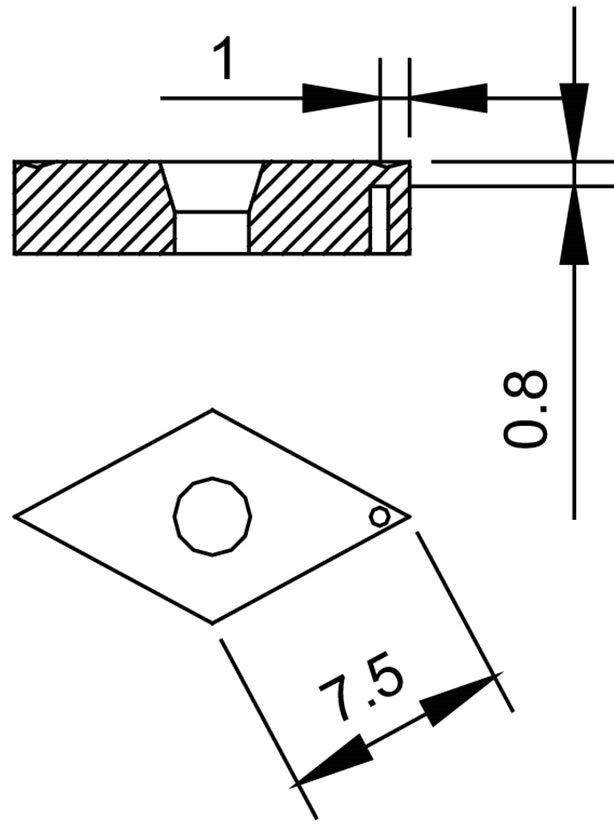
Figure 2. Diamond drilled tungsten carbide insert, type DCMT060202.
A slot was ground into the tool holder to allow a J type thermocouple, 0.5 mm diameter to access the hole in the insert and to be spring loaded against the end of the hole, 0.8 mm from the cutting surface. The lathe and tool were set up to dry machine 6082-T6 aluminium bar 75 mm in diameter and 300 mm long with a tailstock to provide rigid support to the work piece for all tests.
Experiments consisted of setting a depth of cut, the feed/rev and a surface speed and then maintaining the cut until the tool temperature reached a stable value. Figure 3 shows a typical tool temperature—time recording. In this case the stable cutting temperature was 119.6˚C. A series of 96 different cutting trials were performed covering the range of conditions: Cutting speeds, 0.2 - 3.3 m/s; Feed/rev, 0.07 - 0.42 mm; Depth of cut, 0.1 - 1.5 mm. For these conditions, recorded tool temperatures varied from 24˚C to 172˚C. Figures 4-6 show the experimental data obtained for feeds of 0.07, 0.28 and 0.42 mm respectively.
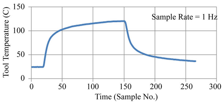
Figure 3. Typical tool temperature-time recording.
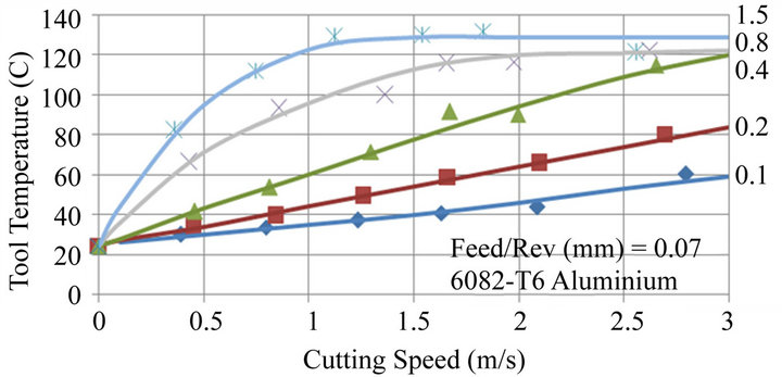
Figure 4. Experiments performed for a 0.07 mm feed/rev and 1.5, 0.8, 0.4, 0.2 and 0.1 mm depths of cut.
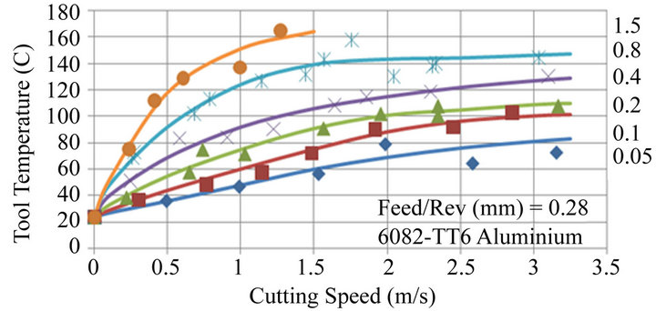
Figure 5. Experiments performed for a 0.28 mm feed/rev and 1.5, 0.8, 0.4, 0.2, 0.1 and 0.05 mm depths of cut.
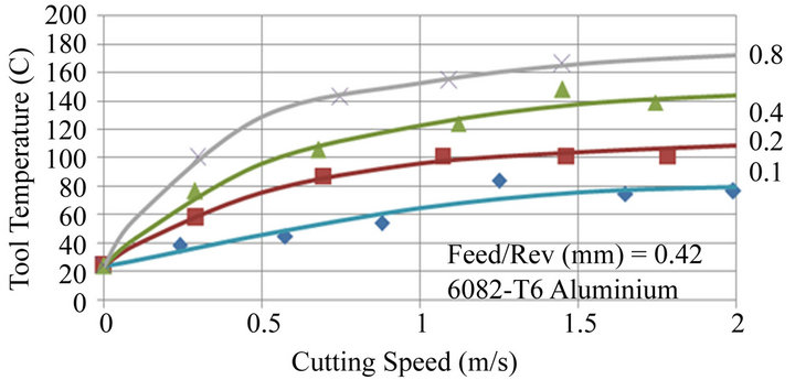
Figure 6. Experiments performed for a 0.42 mm feed/rev and 0.8, 0.4, 0.2 and 0.1 mm depths of cut.
The data exhibited significant scatter. Generally data points were within +/−5˚C of a best fit curve but isolated points, i.e. at 0.28 mm feed/rev, 0.8 mm depth and 1.8 and 2.1 m/s were found to be as much as 16˚C from the curve. The reason for the scatter was attributed mainly to inconsistent swarf clearance. In these experiments a chip breaker was not used and the continuous stream of swarf varied somewhat randomly in path and direction. Occasionally swarf would wrap around the work piece or tool and produce obvious fluctuations in temperature, these experiments are not included in the results. Small temperature measurement errors (estimated at less than 2˚C) also occurred as in practice the tool temperature never reached a perfectly stable value. The bulk temperature of the tool and tool holder continued to rise after the initial rapid transient increase causing the recorded tool tip temperature to continue to increase slowly. The effect of this was minimized by waiting for the rate of increase of tool temperature rate to be less than 1˚C per minute.
Experiments were performed with 4 different work pieces and two tools. Selected experiments, i.e. 0.28 mm feed/rev, 2.3 m/s and 0.8mm and 0.2 mm depth were repeated with the second tool on different work pieces to determine whether tool wear or variation in material properties affected temperature measurements. Within the limits of experimental scatter, agreement with the originnal data suggested neither tool wear nor work piece material was a significant factor in these experiments.
Figures 4-6 clearly show the relationship between tool temperature and cutting speed to be nonlinear, the degree of non linearity increasing with depth of cut. For example at a feed/rev of 0.07 mm and a depth of 1.5 mm tool temperature increases rapidly as speed is increased but reaches a maximum at 1.2 m/s. The same trend is evident at lower depths of cut but a maximum temperature is not reached within the speed range examined.
Figures 7 and 8 are extracted from Figures 4 to 6 and show the dependence of tool temperature on depth of cut and feed rate respectively. The 3 curves in Figure 7 are for cutting speeds of 0.5, 1.0 and 1.5 m/s whilst the 3 curves in Figure 8 are for cut depths of 0.1, 0.2 and 0.4
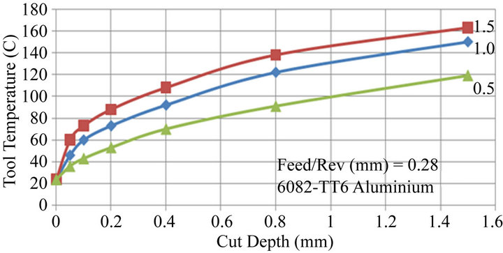
Figure 7. The effect of cut depth on tool temperature for cutting speeds of 1.5, 1.0 and 0.5 m/s.
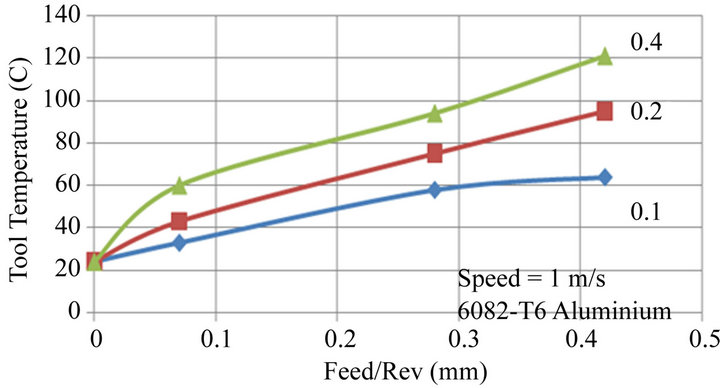
Figure 8. Effect of feed rate on tool temperature for 0.4, 0.2 and 0.1 mm depths of cut.
mm. Both figures show that the relationship between tool temperature and depth of cut or feed rate to be non linear.
3. Optimization of ANN Design
The experimental data in Figures 4-6 was used as a basis for determining an optimum ANN design. The best fit curves to the data shows clearly defined non linear relationships between tool temperature and the machining parameters cutting speed, cut depth and feed rate. But the experimental data points show that superimposed upon the underlying trends there are small but significant random temperature measurement errors. This is broadly attributed to experimental scatter and is a characteristic of machining data. As part of a tool temperature control system, the ANN is required to provide a relationship between tool temperature and machining parameters against which real time tool temperature measurements can be compared and decisions made about the condition of the machining process and what adjustments may be required, if any. Thus, in this application the ANN is required to predict the underlying trends shown in Figures 4-6 and filter out the random temperature measurement errors.
3.1. Application to Data Containing Experimental Scatter
The design algorithm described in [15] was used to optimize the ANN design for this application. A network with a single hidden layer and a TanH activation function was used as a starting point for the work. For the 96 experimental data points of Figures 4-6 the effect of the number of neurons in the hidden layer upon convergence accuracy was determined by systematically varying the number of neurons and finding the minimum convergence error within 100,000 iterations. This was repeated 4 times to assess the repeatability of the convergence process. The results are shown in Figure 9, the curve is the average RMS convergence error and the black lines indicate maximum and minimum values. The convergence process exhibited considerable scatter and the minimum convergence error at 12.8% is considered high. Variation in the convergence process was attributed to the selection of random initial values with which to start the iteration process and the random selection of data points for testing and training. However the extent of the variation and the relatively high convergence error was attributed, at least in part, to experimental scatter within the data points used for training the network. The experimental data in Figures 4-6 show an average error of 7% relative to best fit curves and this must limit the accuracy that the convergence process can achieve.
Figure 10 shows an example of a comparison between ANN predictions and experimental data. This is for a network with 18 neurons in the hidden layer giving a convergence error of 18%. ANN predictions do show the underlying trends in the data but careful inspection of the
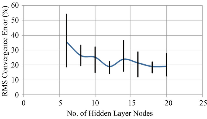
Figure 9. ANN convergence error for experimental data.
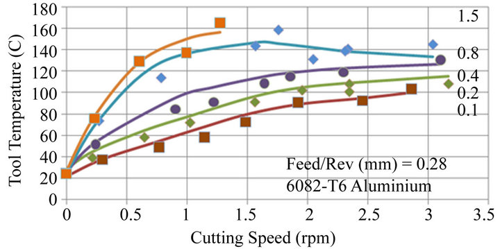
Figure 10. Comparison of ANN predictions and experimental data and 1.5, 0.8, 0.4, 0.2 and 0.1 mm depths of cut.
curves for cut depths of 0.8 and 0.4 mm reveal that the predictions depart from a best fit curve, generally overestimating tool temperature for a given cutting speed. The maximum error is 14.3˚C at a speed of 1.2 m/s and a depth of 0.4 mm.
In applying ANN to machining data subject to experimental scatter it has been found that the training process gives inconsistent convergence errors so that several training exercises may be necessary to find a low convergence error. ANN does however find the under lying trends in the data but even the minimum convergence errors are relatively high and difficult to relate to the accuracy to which predictions fit the real experimental data. Furthermore the optimum number of neurons in the hidden layer is unclear. Figure 9 shows the convergence errors to be most consistent for 12 neurons but similar convergence errors also occur for 18 neurons.
3.2. Application to Filtered Data
Removing experimental scatter from the data by using the best fit curves shown in Figures 4-6 significantly improve the convergence accuracy of the training process.
Figure 11 shows the convergence errors and the consistency of the convergence process for the filtered experimental data to be significantly improved compared to those obtained the raw experimental data. For the TanH activation function used on both sets of data, convergence errors obtained for the filtered data were on average about half of that for the experimental data. Changing the activation function from TanH to Sigmoid gave similar convergence errors for 6 to 14 hidden neurons but a significantly reduced convergence error for 16 to 20 neurons. The lowest average convergence error was 9.3% for 20 neurons and a Sigmoidal activation function. However a network with a hidden layer of 12 neurons and a TanH activation function gave an average convergence error of 9.4% and within the limits of repeatability of the convergence process is considered to be the optimum design.
Figure 12 compares ANN predictions to the filtered data taken from Figure 5. The markers represent the data
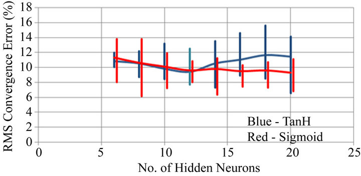
Figure 11. ANN convergence error for filtered data.
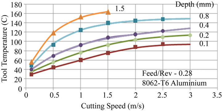
Figure 12. Comparison of ANN predictions and filtered data and 0.8, 0.4, 0.2 and 0.1 mm depths of cut.
whilst the solid lines are ANN predicted trends. The network with a hidden layer of 12 neurons, a TanH activation function and a convergence accuracy of 8.1 % was used for the predictions. Figure 12 is equivalent to Figure 10 but now predicted tool temperatures are within 2˚C of the filtered experimental data. The maximum error for all the data shown in Figures 4-6 is 5˚C occurring locally for a feed/rev of 0.07 mm, a cutting depth of 0.1 mm and a speed of 0.5 m/s.
3.3. Minimum No. of Data Points for Training the ANN
Acquiring experimental data with which to train the ANN can be time consuming. Ninety six data points were obtained to generate Figures 4-6. Seventy eight filtered data points were used to train the network corresponding to Figure 12. On the assumption that reliable and consistent experimental data can be obtained by for example, repeating the same cut condition and averaging temperature measurements, then knowing how convergence error depends upon the number of data points used for training can help to minimise experimental work.
The filtered data corresponding to Figure 12 was assumed to be representative of experimental data not subject to significant experimental scatter. The original 78 data points were reduced to 55 points by eliminating the 0.5 m/s and 2.0 m/s speed conditions and then to 36 points by also eliminating the 0.2 mm and the 0.8 mm depths of cut. All 3 sets of data were used to train the optimised ANN having a single hidden layer of 12 neurons. For each set of data the ANN was trained 5 times to determine the minimum convergence error. Table 1 shows how the minimum convergence error depends on the number of data points.
The results show convergence error to steadily increase as the number of points used for training decreases. An example of the effect of this upon tool temperature predictions is shown in Figure 13 where for 36 data points and a 0.28 mm/rev feed rate, ANN predictions are compared with the filtered data of Figure 12. Whereas for Figure 12 ANN predictions based on 78 training data
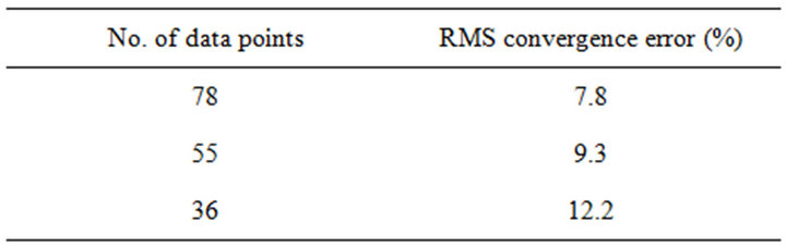
Table 1. Minimum convergence error v No. of training data points.
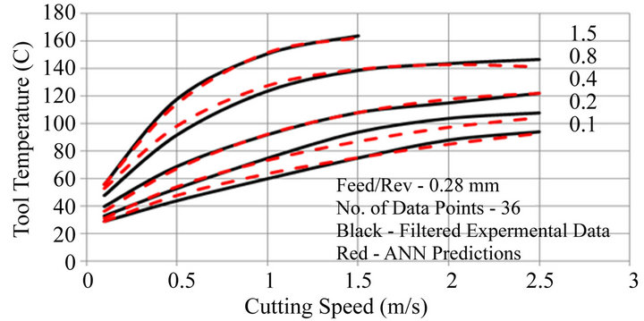
Figure 13. Example of ANN predictions for 36 training data points depths of cut—1.5, 0.8, 0.4, 0.2 and 0.1 mm.
points are within 2˚C of the filtered experimental data, the error has increased to 8˚C for 36 data points. This error is for the 0.28 mm feed/rev, the maximum error over the full range of test conditions used for Figures 4- 6 was 11˚C, about the maximum acceptable in this application.
3.4. Reduced Range of Cutting Conditions
Not every machining application needs to embrace a wide range of cutting conditions. Where only a narrow range of conditions are being used, a further reduction in the number of data points required for training the ANN is of interest.
Reducing the range of the machining conditions effectively reduces the degree of non linearity exhibited by the experimental data and it is reasonable to expect to be able to reduce the number of data points required for training the ANN without compromising convergence error. The original seventy eight filtered data points were reduced by first eliminating maximum and minimum speed conditions and then by also eliminating maximum and minimum depths of cut. The feed rates of 0.07, 0.28 and 0.42 mm/rev were retained. The effect of the number of data points used for training upon RMS convergence error for an ANN with a single hidden layer of 12 neurons and a TanH activation function is shown in Table 2. RMS convergence error tabulated is the minimum over 5 training processes and is shown to generally decrease with reduced number of data points and parameter range. An example of the effect of this on tool temperature predictions is shown in Figure 14.
For 55 data points and the cutting speed range reduced
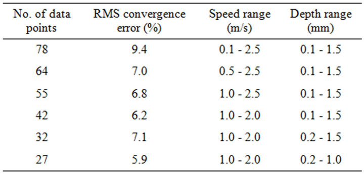
Table 2. Convergence error v No. of data points for reduced parameter range.
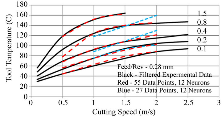
Figure 14. Effect of reduced parameter range on ANN predicted tool temperatures for 1.5, 0.8, 0.4, 0.2 and 0.1 mm depths of cut.
to 0.5 - 2.0 m/s the tool temperature predictions are accurate with one exception—the 0.5 m/s, 0.8 mm depth shows an error of 14˚C. For 27 data points and the speed range reduced to 1.0 - 2.0 m/s and depth of cut reduced to 0.2 - 0.8 mm the predictions are generally less accurate showing errors of 13˚C and 8˚C at a cutting speed of 2.0 m/s and depths of 0.8 and 0.4 mm respectively. The RMS convergence errors were similar at 6.8% for 55 and 5.9% for 27 data points. For both examples the ANN prediction accuracy in terms of absolute cutting tool temperature is of concern as in this application it is required to have a reasonable accuracy over a full range of conditions rather than good accuracy over most of the range combined with high local errors. The predictions have also failed to preserve the non linear trends exhibited by the data even though the range of the data and hence the degree of non linearity has been reduced.
In reducing the range of the experimental parameters, the characteristics of the data are also being changed and it follows that ANN design containing a single layer of 12 neurons, optimized over the full range of experimental conditions may no longer be appropriate. For the reduced parameter ranges shown in Figure 14 the ANN design was re-optimized. For 55 data points a single hidden layer of 8 neurons produced a minimum convergence error of 5.3% whereas for 27 data points a single hidden layer of 5 neurons gave a minimum error of 3.9%. Both networks retained the TanH activation function used previously. The results are shown in Figure 15 and in both cases the ANN predictions in terms of absolute tool temperature are greatly improved over those shown in Figure 14. For 27 data points prediction accuracy was within 1˚C over the full range of conditions. The improved prediction accuracies are accompanied by much faster convergence times.
3.5. Application to Internally Cooled Tools
The set up shown in Figure 1 was used to generate experimental data for assessing the application of artificial neural networks to internally cooled tools. The machine tool was an Alpha Colchester Harrison 600 Group CNC lathe. The tool is a composite design comprising of a tool holder with integrated inlet and outlet tubes, a cooling block with integrated cooling geometry and a wear resistant insert made from tungsten carbide [ref: 20. Sun 2011]. The tool insert is a hollow shell with a fixed wall thickness which fits over the top of the cooling block, this allows the coolant to be pumped through the tool holder and pass close to the tool tip before being returned to the closed loop coolant supply. The insert was made by taking a standard SPUN type insert and using the EDM process to remove material to form the hollow. It should be noted that the inserts also have a TiN coating. The work piece was a cylindrical bar nominally 62 mm diameter and 300 mm long manufactured from AA6082- T6 aluminium. A tailstock was used to provide rigid support of the work piece for all trials. As the internal cooling circuit made it difficult to locate a thermocouple close enough to the tool tip to record a temperature representative of the cutting process an optical pyrometer, µ-Epsilon, model CTLM3- H1 CF2, was used to measure chip temperature. The pyrometer was mounted to the tool turret within the machine tool to maintain a minimum spot size of 0.45 mm at a constant working distance of 150 mm. It should be noted that any relevant parameter can be used to control tool temperature utilizing artificial neural networks. Even with a direct tool temperature measurement a transfer function will still be required to
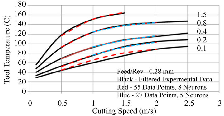
Figure 15. The effect of reduced parameter range and reoptimised ANN on tool temperature predictions for 1.5, 0.8, 0.4, 0.2 and 0.1 mm depths of cut.
relate the actual measurement to the cutting edge temperature. Thus in principle it doesn’t matter what the parameter is.
Of primary interest in this assessment was to find out whether a relatively low number of experimental data points could be used to train the artificial neural network for controlling tool (chip) temperature over a relatively low range of cutting conditions. Depth of cut was limited to between 0.2 and 0.5 mm; feed/rev to between 0.1 and 0.2 mm and cutting speed to between 250 and 350 m/min. Experiments were performed with zero (dry cutting) and 0.3 l/min coolant flow rates. For each of these cooling conditions 27 data points were used to optimize and train the neural network. To minimize experimental scatter machining trials at each cutting condition were performed 3 times and the recorded temperature checked for consistency. Extraneous measurements were discarded and the trial repeated. A network with a single hidden layer of 7 neurons and a TanH activation function was found to provide convergence errors of less than 5%. The accuracy to which predicted tool (chip) temperatures fit the experimental data is shown in Table 3. The maximum error is less than 5˚C and is generally within 2˚C for temperatures in the range 188˚C to 258˚C.
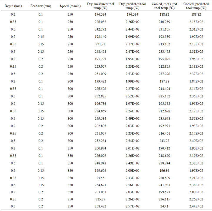
Table 3. Experimental and predicted temperature measurements for an internally cooled tool.
4. Discussion
In practice tool temperature measurements for given machining conditions are prone to variation due to a number of extraneous effects. For the experiments performed in this investigation the lack of a chip breaker was a primary cause of apparently random tool temperature variations that are broadly referred to as experimental scatter. In using such data for training and optimizing ANN’s it was found that minimum RMS convergence errors were large, in excess of 11%, and that the convergence process was inconsistent, exhibiting large variations in minimum convergence error. Nonetheless, the experimental data enabled an optimum design of ANN to be determined and this successfully predicted the underlying trends within the data as shown in Figure 10.
For the 3 input variables: cutting speed, depth and feed/rev and the parameter range investigated the optimum design of ANN had a single layer of 12 neurons and a TanH activation function. The latter was found to produce marginally lower convergence errors than a Sigmoidal activation function for less than 14 hidden neurons whereas for 16 - 20 hidden neurons the Sigmoidal function produced the lower convergence errors. Only a single hidden layer of neurons was considered as prior investigations, [17] have shown that it is the total number of hidden neurons that determine convergence error and not the number of hidden layers that they may be distributed within.
With the presence of experimental scatter and for the parameter range investigated, the 96 experimental data points were found to be sufficient for training and optimizing ANN design. In this case, there were enough data points to enable the ANN to average out experimental scatter and find the underlying trends. However, if it is required to minimize the number of data points used for training then scatter must be reduced to a negligible level to give a high degree of confidence in the data’s integrity. This may be achieved by attention to experimental detail but in this investigation the experimental data was effectively filtered by using best fit curves. Using 78 filtered data points for optimizing and training the ANN also resulted in a network with 12 hidden neurons and a TanH activation function and this gave good agreement between ANN predictions and the filtered data as shown in Figure 12. Furthermore the convergence process was found to be more consistent.
Maintaining the parameter range and further reducing the number of data points used for training the ANN steadily increased the minimum convergence error that could be achieved. Figures 12 and 13 show that for the same data, maximum errors between ANN predictions and filtered experimental data increased from 2˚C to 8˚C when the number of points used for training decreased from 78 to 36.
Reducing the parameter range together with the number of data points used for training but maintaining the optimized 12 hidden neuron network produced lower RMS convergence errors. However the errors tended to be localized so that although the RMS error was low for all data points, individual errors were high. The effect was that ANN predictions did not accurately reproduce the underling trends in the data as shown in Figure 14.
Reducing the parameter range together with the number of data points and re-optimizing the ANN design produced good agreement between ANN predictions and the filtered data as shown in Figure 15. For 27 data points tool temperature predictions were within 1˚C of the filtered data, albeit for cutting speeds limited to between 1 and 2 m/s and depths to between 0.2 and 0.8 mm. The optimum ANN had only 5 neurons in a single hidden layer and produced rapid convergence. 27 data points was the minimum used in this investigation as it allowed each of the 3 input parameters to have 3 independent values—the minimum necessary to characterize non linear data.
The above findings were verified using an internally cooled tool and measuring chip temperature with an optical pyrometer. 27 experimental data points were used to train and optimize an ANN for a limited range of cutting conditions, depth: 0.2 - 0.5 mm, feed/rev: 0.1 - 0.2 mm and speed: 250 - 350 m/min. The optimum ANN had a single hidden layer of 7 neurons and predicted temperatures to within 5˚C for measured temperatures in the range 188˚C - 258˚C.
5. Conclusions
1) ANN’s can be used to predict the underlying nonlinear trends in tool temperature data obtained over a range of machining conditions, even when experimental scatter is present.
2) However ANN predictions are more accurate and fewer data points are required for training if experimental scatter is reduced or eliminated.
3) The optimum ANN design, the number of experimental data points required for training and the range of the data are interrelated. Wide ranging data requires an ANN with a relatively large number of hidden neurons and many experimental data points whereas for data obtained over a narrow range of conditions an ANN with a low number of hidden neurons and few experimental data points can provide accurate predictions.
4) The findings based on dry machining with conventional tool designs apply to internally cooled tool designs.
6. Acknowledgements
The authors gratefully acknowledge the European Commission for funding and supporting the ConTemp project of which this work is part. The authors also extend their gratitude to all ConTemp partners for their constructive contributions to the control system development.
REFERENCES
- E. Uhlmann and M. Roeder, “Internal Cooling of Cutting Tools,” Lambda Map Conference, London, July 2009.
- F. Klocke, “Dry Cutting, Keynote Paper,” Annals of the CIRP, Vol. 46, No. 2, 1997, pp. 519-526.
- V. P. Astakhov, “Effects of the Cutting Feed, Depth of Cut, and Workpiece (Bore) Diameter on the Tool Wear Rate,” International Journal of Advanced Manufacturing Technology, Vol. 34, No. 7-8, 2007, pp. 631-640.
- E. Dimla Jr., P. E. Lister and N. J. Leighton, “Neural Network Solutions to the Tool Condition Monitoring Problem in Metal Cutting—A Critical Review of Methods,” International Journal of Machine Tools and Manufacture, Vol. 37, No. 9, 1997, pp. 1291-1241.
- D. A. Dornfield, “Neural Network Sensor Fusion for Tool Condition Monitoring,” Annals CIRP, Vol. 39, No. 1, 1990, pp. 101-105. doi:10.1016/S0007-8506(07)61012-9
- T. I. Liu and E. J. Ko, “On-Line Recognition of Drill Wear via Artificial Neural Networks,” Winter Annual Meeting of the ASME, Monitoring and Control for Manufacturing Processes, Vol. 44, Dallas, 1990, p. 101.
- S. Purushothaman and Y. G. Srinivasa, “A Back Propogation Algorithm Applied to Tool Wear Monitoring,” International Journal of Machine Tools and Manufacture, Vol. 34, No. 5, 1994, pp. 625-631.
- Q. Liu and Y. Altintas “On-Line Monitoring of Flank Wear in Turning with Multilayered Feed-Forward Neural Networks,” International Journal of Machine Tools and Manufacture, Vol. 39, No. 12, 1994, pp. 1945-1959. doi:10.1016/S0890-6955(99)00020-6
- L. I. Burke and S. Rangwala, “Tool Condition Monitoring in Metal Cutting: A Neural Network Approach,” Journal of Intelligent Manufacturing, Vol. 2, No. 5, 1991, pp. 269-280. doi:10.1007/BF01471175
- L. I. Burke, “Competetive Learning Approaches to Tool Wear Identification,” IEEE Transactions on System, Man and Cybernetics, Vol. 22, No. 3, 1992, pp. 559-563.
- A. Ruiz, D. Guinea, J. Barrios and F. Betancourt, “An Empirical Multi-Sensor Estimation of Tool Wear,” Mechanical Systems and Signal Processing, Vol. 7, No. 2, 1993, pp. 105-119.
- Q. Zhou, G. S. Hong and M. Rahman, “A New Tool Wear Criterion for Tool Condition Monitoring using Neural Networks,” Engineering Applications of Artificial Intelligence, Vol. 8, No. 5, 1995, pp. 579-588. doi:10.1016/0952-1976(95)00031-U
- Q. Zhou, G. S. Hong and M. Rahman, “On-Line Cutting State Recognition in Turning Using a Neural Network,” International Journal of Advanced Manufacturing Technology, Vol. 10, No. 2, 1995, pp. 87-92. doi:10.1007/BF01179276
- Q. Zhou, G. S. Hong and M. Rahman, “Using Neural Networks for Tool Condition Monitoring Based on Wavelet Decomposition,” International Journal of Machine Tools and Manufacture, Vol. 36, No. 5, 1996, pp. 551-566. doi:10.1016/0890-6955(95)00067-4
- M. Guillot and A. El Ouafi, “On-Line Identification of Tool Breakage in Metal Cutting Processes by Use of Artificial Neural Networks,” Proceedings of ANNIE 91, St Louis, 10 November 1991, p. 701.
- Y. I. Yao and X. Fang, “Assessment of Chip Forming Patterns with Tool Wear Progression in Machining via Neural Networks,” International Journal of Machine Tools and Manufacture, Vol. 33, No. 1, 1993, pp. 89-102.
- S. Zurek, A. J. Moses, M. Packianather, P. Anderson and F. Anayi, “Prediction of Power Loss and Permeability with the Use of an Artificial Neural Network in Wound Toroidal Cores,” Journal of Magnetism and Magnetic Materials, Vol. 320, No. 20, 2008, pp. 1001-1005.
- S. Y. Liang, et al., “Machining Process Monitoring and Control: The State-of-the-Art,” Journal of Manufacturing Science and Engineering, Vol. 126, No. 2, 2004, pp. 297- 310.
- M. A. Davies, et al., “On the Measurement of Temperature in Material Removal Processes,” Annals of CIRP, Vol. 56, No. 2, 2007, pp. 581-604.
- X. Sun, R. Bateman, K. Cheng and S. C. Ghani, “Design and Analysis of an Internally-Cooled Smart Cutting Tool for Dry Cutting,” Journal of Engineering Manufacture, 2011.