Journal of Power and Energy Engineering
Vol.04 No.01(2016), Article ID:62374,39 pages
10.4236/jpee.2016.41001
On the Maximum of Wind Power Efficiency
Gerhard Kramm1*, Gary Sellhorst2, Hannah K. Ross3, John Cooney4, Ralph Dlugi5, Nicole Mölders6
1Engineering Meteorology Consulting, Fairbanks, USA
2Geophysical Institute, University of Alaska Fairbanks, Fairbanks, USA
3Department of Mechanical Engineering, University of Washington, Seattle, USA
4Department of Atmospheric Sciences, Texas A & M University, College Station, USA
5Arbeitsgruppe Atmosphärische Prozesse (AGAP), Munich, Germany
6College of Natural Science and Mathematics and Geophysical Institute, University of Alaska Fairbanks, Fairbanks, USA

Copyright © 2016 by authors and Scientific Research Publishing Inc.
This work is licensed under the Creative Commons Attribution International License (CC BY).
http://creativecommons.org/licenses/by/4.0/


Received 7 October 2015; accepted 26 December 2015; published 29 December 2015
ABSTRACT
In our paper we demonstrate that the filtration equation used by Gorban’ et al. for determining the maximum efficiency of plane propellers of about 30 percent for free fluids plays no role in describing the flows in the atmospheric boundary layer (ABL) because the ABL is mainly governed by turbulent motions. We also demonstrate that the stream tube model customarily applied to derive the Rankine-Froude theorem must be corrected in the sense of Glauert to provide an appropriate value for the axial velocity at the rotor area. Including this correction leads to the Betz-Joukowsky limit, the maximum efficiency of 59.3 percent. Thus, Gorban’ et al.’s 30% value may be valid in water, but it has to be discarded for the atmosphere. We also show that Joukowsky’s constant circulation model leads to values of the maximum efficiency which are higher than the Betz-Jow- kowsky limit if the tip speed ratio is very low. Some of these values, however, have to be rejected for physical reasons. Based on Glauert’s optimum actuator disk, and the results of the blade-ele- ment analysis by Okulov and Sørensen we also illustrate that the maximum efficiency of propeller- type wind turbines depends on tip-speed ratio and the number of blades.
Keywords:
Wind Power, Power Efficiency, General Momentum Theory, Axial Momentum Theory, Blade Element Analysis, Betz-Joukowsky Limit, Joukowsky’s Constant Circulation Model, Glauert’s Optimum Actuator Disk, Balance Equation for Momentum, Equation of Continuity, Balance Equation for Kinetic Energy, Reynolds’ Average, Hesselberg’s Average, Favre’s Average, Bernoulli’s Equation, Integral Equations

1. Introduction
In 2001, Gorban’ et al. [1] challenged the Betz limit (in our study called the Betz-Joukowsky limit [2] - [6] even though it has also been denoted as Lanchester-Betz-Joukowsky limit [2] [6] ), i.e., the maximum power efficiency of 59.3 percent for a propeller-type turbine, where the power efficiency is generally defined by
 . (1.1)
Here, P is the extracted (or consumed) power, and  is the power carried by the flow through the projection of the turbine section region onto the plane perpendicular to it. Gorban’ et al. [1] argued that the maximum efficiency of the plane propeller is about 30 percent for free fluids. Meanwhile, their paper has been cited numerous times in conference papers (e.g., [7] [8] ), but recently van Kuik et al. [9] rejected their method and pointed out that the main problem of Gorban’ et al. “is their lack of comprehension of the working principles how the turbine operates”. Since this argument is very harsh, it is indispensable to show that the result of Gorban’ et al. is based on an equation that may be acceptable for water fluids of low flow velocity, but that is indeed not very suitable for flows as they are typical in the atmospheric boundary layer (ABL, the lowest layer of the troposphere, with a thickness of the order of
 ), especially at heights between 30 m to 150 m above the Earth’s surface.
According to Gorban’ et al. [1] , the filtration equation,
 , (1.2)
holds in an open domain  (denoted by [1] as
 ) with a smooth or piecewise smooth boundary together with the equation of continuity,
  (only valid for an incompressible stationary flow), where p and
  denote the pressure and the velocity of the flow, respectively. The shape of
  is considered as a semi-penetrable obstacle for the stream with a resistance density r inside. Let
  the cross section of
  perpendicular to the flow axis. The power carried by the flow through
  is then given by
 . (1.3)
Following these authors,  is the velocity of a uniform laminar current. Gorban’ et al. [1] argued that the power, P, consumed by the turbine is given by
 , (1.4)
where the filtration Equation (1.2) has been inserted. In accord with Equation (1.1), they obtained
 . (1.5)
Gorban’ et al. [1] claimed:
“The efficiency coefficient can be maximized by optimizing the resistance density. The optimal ratio between the streamlining current and the current passing through the turbines can also be obtained from this model. This parameter can be measured experimentally to determine how close a real turbine is to the theoretically optimal one.”
Obviously, the maximum of the efficiency coefficient deduced by Gorban’ et al. [1] depends on the filtration equation. This equation, however, plays no role in the description of ABL flows. In addition, the ABL is mainly governed by turbulent motions. If we assume, for instance, a wind speed of  at a hub height of
  and a kinematic viscosity of
  we will obtain a Reynolds number of about
 . (1.6)
This Re value is far beyond the critical Reynolds number at which the transition from a laminar to a turbulent flow occurs.
In the following section, we will present the governing equations for macroscopic and turbulent systems relevant for wind power studies: (a) the local balance equations for momentum (also called the Navier-Stokes equation), (b) total mass (also called the equation of continuity), and (c) kinetic energy. It is shown that the Bernoulli equation for an incompressible flow can simply be derived from the local balance equation of kinetic energy. Furthermore, we will derive the simplified integral balance equations recently used by Sørensen [6] in his review on the aerodynamic aspects of wind energy conversion to incorporate his results in our discussion. Additionally, we will demonstrate that Equation (1.4) derived by Gorban’ et al. [1] is incomplete for the ABL so that their maximum efficiency calculation for plane propellers of about 30 percent for free fluids has to be discarded, as suggested by van Kuik et al. [9] . This means that the filtration Equation (1.2) is meritless if the maximum efficiency of wind power has to be determined. In Section 3, we will discuss the main characteristics of propeller-type wind turbines. Our discussion will include the basics of the axial momentum theory, Joukowsky’s constant circulation model, Glauert’s infinite-bladed actuator disk model, and finite-bladed rotor models. We will show that the Betz-Joukowsky limit is, indeed, the maximum of the wind power efficiency, even though some results of Joukowsky’s constant circulation model might exceed it because of physically inadequate conditions. Glauert’s [10] optimum actuator disk and finite-bladed rotors [6] [11] [12] tend to this maximum, if the tip- speed ratio,  , increases.
2. Theoretical Background
2.1. The Governing Equations for the Macroscopic System
In order to outline the generation of electricity by extracting kinetic energy from the wind field we consider the local balance equations for momentum (i.e., Newton’s 2nd axiom), Equation (2.1), and total mass, Equation (2.2), for a macroscopic system given by (e.g., [13] -[16] ):
 (2.1)
(2.1)
and
 . (2.2)
Here,  is the air density, t is time,
  is the velocity of the flow,
  is the Stokes stress tensor given by
 . (2.3)
where  is the bulk viscosity (near zero for most gases),
  is the identity tensor,
  is the gravity potential, and
  is the angular velocity of the Earth. Both
  and
and  are symmetric second-rank tensors. Furthermore, the 1st term of the left-hand side of Equation (2.1) describes the local temporal change of momentum, and the 2nd term represents the exchange of momentum between the system under study and its surroundings, where
  exerts on the boundary of this system. The 1st term on the right-hand side of this equation represents the gravity force, and the 2nd one the Coriolis force. Equation (2.2) is the equation of continuity. In addition, local balance equations for various energy forms (i.e., internal energy, kinetic energy, potential energy, and total energy), various water phases (i.e., water vapor, liquid water, and ice), and gaseous and particulate atmospheric trace constituents exist. All these local balance equations can be derived from integral balance equations (e.g., [13] [14] ). Since
  and
and , Equation (2.1) is often written as (e.g., [17] - [19] )
 , (2.4)
where  is the substantial derivative with respect to time. This equation form not only disguises its origin, namely the corresponding integral balance equation, but also is unfavorable if it has to be averaged, for instance, in the sense of Reynolds [20] to find a tractable equation for turbulent atmospheric layers. Nevertheless, in accord with Lamb’s transformation (e.g., [21] )
 , (2.5)
Equation (2.4) may be written as
 . (2.6)
The curl of Equation (2.6) leads to the prognostic equation for the vorticity
 , (2.7)
As the curl of the gradient of a scalar field is equal to zero, Equation (2.7) can be written as
 . (2.8)
This equation plays an important role in the description of rotational flows as occurred in the wake of the wind turbine. If the friction effect is negligible and the density is considered as spatially constant like in case of an incompressible fluid we will obtain
 . (2.9)
To deduce the local balance equation for the kinetic energy of the flow, Equation (2.1) has to be scalarly multiplied by the velocity vector . Using the identities
 (2.10)
and
 (2.11)
leads to
 . (2.12)
The colon expresses the double-scalar product (also called the double dot product) of the tensor algebra. Furthermore, . The 1st term of the left-hand-side of Equation (2.12) describes the local temporal change of kinetic energy, and the 2nd term is the energy exchange of the system with its surroundings which is performed by the surrounding air on the boundary of the system. The 1st term of the right-hand-side represents the conversion of potential energy into kinetic energy and vice versa, the 2nd term describes the reversible work rate of expansion,
  , or contraction,
  , and the 3rd term represents the irreversible work rate owing to viscous friction. This term represents the dissipation of kinetic energy into the reservoir of heat. The term of our primary interest reads
 . (2.13)
It describes the transport of kinetic energy by the flow, and it may be called the kinetic energy stream density, but it is also denoted as wind power density. Inserting the definition of the total pressure,
 , (2.14)
into Equation (2.12) yields
 . (2.15)
2.2. The Governing Equations for the Turbulent System
Since the ABL is mainly governed by turbulent motion, the use of the macroscopic balance Equations (2.1), (2.2), and (2.12) is rather impracticable. Therefore, these balance equations are customarily averaged in the sense of Reynolds [20] . However, conventional Reynolds averaging will lead to various short-comings in the set of governing equations for turbulent atmospheric flow, even if these averaging techniques can be performed accurately [22] . If we ignore, for instance, density fluctuation terms, the possibility to describe physical processes as a whole will clearly be restricted (see [23] [24] ). The key questions that still remain are (a) how to average the governing macroscopic equations in the case of turbulent atmospheric flows and (b) what are the consequences of such an averaging, not only for momentum and total mass, but also for various energy forms like kinetic energy, potential energy, internal energy, and total energy, consisting of the sum of these three energy forms. In the terrestrial atmosphere, the total energy is conserved. As sketched in Figure 1 for a turbulent system (Hesselberg fluid), there are various ways of energy conversion.
As argued by various authors [22] -[34] , the density-weighted averaging procedure suggested by Hesselberg [35] is very appropriate to formulate the balance equation for turbulent systems. It is given by
 , (2.16)
where  is a field quantity like the wind vector,
  , the specific internal energy, e, and the specific enthalpy, h. Furthermore, the overbar (
 ) characterizes the conventional Reynolds mean. Whereas the hat (
 ) denotes the density-weighted average according to Hesselberg, and the double prime (") marks the departure from that. It is
obvious that . The Hesselberg mean of the wind vector, for instance, is given by
 .
.
Note that intensive quantities like the pressure, p, and the density,  , of air are averaged in the sense of Reynolds. Arithmetic rules can be found, for instance, in [25] - [27] [29] [31] . As pointed out by Kramm and Meixner [22] and Lumley and Yaglom [36] , Hesselberg’s average is sometimes misnamed the Favre average.
In comparison with that of Reynolds, Hesselberg’s averaging calculus leads to several prominent advantages [22] [25] - [27] [29] - [31] [35] : (a) The equation of continuity,

Figure 1. Schematic representation of the energy conversion within a turbulent system (Hesselberg fluid) and the exchange of energy with its surroundings which is performed by the surrounding air on the boundary of the system. As illustrated in this sketch, there is no direct conversion of mean internal energy into mean potential energy and vice versa. Note that  is the total irradiance, where RS is solar irradiance and RIR is the infrared irradiance. Furthermore,
  and
and  are the mean molecular and the turbulent enthalpy flux densities, respectively. All other symbols are explained in the text.
 , (2.17)
keeps its form, and (b) the mean value of kinetic energy can exactly be split into the kinetic energy of the mean motion and mean value of the kinetic energy of the eddying motion, according to
 . (2.18)
This advantage is especially important in the theoretical description of the extraction of the kinetic energy from the wind field for generating electricity. The use of density-weighted averages is the common way to define averages in studies of highly compressible turbulent flows (see also [29] [32] ), probably the most natural way to define averages. The kinetic energy of the mean motion is usually abbreviated by MKE, and the kinetic energy of the eddying motion is usually called the turbulent kinetic energy abbreviated by TKE.
Hesselberg’s average procedure will be applied within the framework of this contribution. It can be related to that of Reynolds by (e.g., [22] [26] [30] [31] [37] )
 . (2.19)
Here, the prime ( ) denotes the deviation from the Reynolds mean. Obviously, the different means,
  and
and
 , are nearly equal if
  as used, for instance, in case of the Boussinesq approximation. In case
of a nearly incompressible fluid, the distinction between  and
and  is not necessary because the condition
 is clearly fulfilled. However, to avoid any kind of confusion, we keep our notation.
In the averaged form, the local balance equation for momentum of the turbulent atmosphere reads (e.g., [22] [25] - [27] [29] [35] [38] )
 , (2.20)
where  is the Reynolds stress tensor. It results from averaging the term
  in Equation (2.1) leading to
 . Similar local balance equations can be derived for various energy forms (i.e.,
internal energy, kinetic energy, potential energy, and total energy), various water phases (i.e., water vapor, liquid water, and ice), and gaseous and particulate atmospheric trace constituents [22] [25] - [31] [38] [39] .
Averaging Equation (2.12) provides the corresponding local balance equation for the kinetic energy
 (2.21)
Obviously, the local derivative with respect to time not only contains the MKE, but also the TKE as outlined by Equation (2.18). Assuming, for instance, steady-state condition leads to
 (2.22)
This means that the total kinetic energy is time-invariant, but MKE can be converted into TKE. In the inertial range, for instance, the TKE is transferred from lower to higher wave numbers until the far-dissipation range is reached, where kinetic energy is converted into heat energy by direct dissipation,  , and turbulent dissipa-
tion, . Even though the fluctuations of the wind vector are usually small as compared to the mean wind vector,
  , the opposite is true for their gradients,
 . This phenomenon is connected with a
great intensity of rotation and is characteristic for all turbulent flows. Except for the immediate vicinity of rigid walls, turbulent dissipation exceeds direct dissipation by several orders of magnitude depending on the Reynolds number (e.g., [18] [22] ). Furthermore, the mean kinetic energy stream density reads
 . (2.23)
This equation describes the transfer of MKE and TKE by the mean wind field and the transfer of TKE by the eddying wind field. Ignoring the turbulent effects yields
 , (2.24)
i.e.,  is approximated by the MKE stream density. The magnitude of
  is given by
 , (2.25)
where . Apparently, this quantity expresses that the wind power density is proportional to the cube of the wind speed. The rotor of a wind turbine causes a divergence effect expressed by
 .
.
Unfortunately, there is a notable inconsistency regarding the role of the turbulence intensity. According to de
Vries [40] , for instance, this quantity is , where
  is the standard deviation of the horizontal wind
speed and  is the corresponding variance. If we assume that only a horizontal component of the mean wind field exists, for the purpose of convenience, in the direction of the x-axis of a Cartesian coordinate frame, Equation (2.23) would provide
 (2.26)
or
 , (2.27)
i.e. we have still to consider the fluctuations of all components in this coordinate frame. On the other hand, de
Vries [40] argued that the instantaneous value is given by , and, hence,
  , i.e.,
 . (2.28)
Since , we have
 . (2.29)
The term  is only equal to zero when the probability distribution of u is symmetrical. Nevertheless,
for estimating the effect owing to turbulence this term is ignored which leads to
 . (2.30)
Ignoring the similar term in Equation (2.27) yields
 , (2.31)
where  and
and  are the variances with respect to the y- and z-axis of a Cartesian coordinate frame. Thus, only in case of
  Equations (2.30) and (2.31) become identical, but such an equality does not generally exist. Figure 2 shows that the mean and the median of the turbulence intensity depending at the height of 90 m [41] . The observations were performed at the offshore measurement platform FINO1 which is located 45 km north of the island of Borkum in the German Bight. For wind speeds ranging from
  to
to  the mean and the median of the turbulence intensity are smaller than 0.1. This means that according to Equation (2.30), the effects of the turbulence intensity are smaller than 3 percent. As reported by Türk and Emeis [41] , the same is true for this wind speed range at the 30 m height. The effect by turbulence may become more influential in case of aerodynamically rougher landscapes covered, for instance, with vegetation. In case of wind farms the effect by turbulence may considerably increase inside the array of wind turbines [42] [43] .
To obtain the local balance equation of MKE, Equation (2.20) has to be scalarly multiplied by  leading to
 (2.32)
or
 (2.33)
with
 . (2.34)
The quantity H may be considered as the mean total pressure. Subtracting Equation (2.32) from Equation (2.21) yields
 (2.35)
or
 , (2.36)

Figure 2. Turbulence intensity depending on wind speed at 90 m height for the period September 2003-August 2007 (taken from Türk and Emeis, [41] ). The observations were performed at the offshore measurement platform FINO1 which is located 45 km north of the island of Borkum in the German Bight.
where
 (2.37)
is a non-dimensional parameter characterizing the thermal stability of a turbulent flow. This stability parameter expresses the relative importance of the two TKE-terms. It may be interpreted as a generalized Richardson number. The difference between the well-known flux-Richardson number and the generalized Richardson number results from the parameterization of  [22] [27] . Besides the vertical effects also horizontal effects have to be regarded under certain circumstances. In case of
 , mechanically produced TKE is mainly consumed by Archimedean effects. Consequently, there exists a critical
  -value given by
 . It characterizes that the mechanical gain of TKE is equal to the thermal loss of TKE, i.e., the term
 becomes equal to zero, and the net production rate of TKE vanishes. As the turbulent dissipation still acts as a sink of TKE, the turbulent flow will become more and more viscous (laminar). In case of
 , TKE is generated mechanically and thermally. If the mechanically generated TKE is much smaller than the thermal gain of TKE, and, hence, negligible, free convective conditions,
  , will occur. In the remaining range, forced convective conditions may prevail,
 . Thermally neutral stratification is characterized by
 . The 2nd-order balance equation (2.35) is the only balance equation that additionally arises from averaging a macroscopic balance equation (e.g., [18] [23] ). In meteorological models, the balance equation of TKE (2.35) serves to derive the eddy diffusivities for momentum and―via the turbulent Prandtl number and the species-dependent turbulent Schmidt numbers―the eddy diffusivities for sensible heat, and water vapor. This method of parameterization is known as one-and-a-half-order closure (e.g. [22] [44] [45] ). In the mesoscale model of the National Centers for Environmental Prediction (NCEP) and the Weather Research and Forecasting (WRF) model, it is realized with respect to the level 2.5 of Mellor and Yamada [46] - [48] .
The local balance equation for the mean total energy  can be deduced from Figure 1 leading to
 . (2.38)
This equation demonstrates that no production or destruction of mean total energy within any given fixed volume exists (e.g., [22] [26] [27] [29] ). Obviously, contributions of energy of different orders of magnitude are summed, where only a very small fraction of the total potential energy (or total internal energy),  , is available for conversion into kinetic energy (e.g., [22] [49] - [52] ).
From the perspective of the generation of electricity by extracting kinetic energy from the wind field, Equations (2.17), (2.20), and (2.32) play the dominant role. To obtain a tractable set of equations, effects caused by
molecular and turbulent friction,  ,
,  , and
, and , are usually ignored. In addition, incompressibility (
 ) and steady state (
 ) conditions are presupposed. In doing so, the set of
approximated equations reads
 , (2.39)
 , (2.40)
and
 . (2.41)
2.3. The Bernoulli Equation
Because of the condition of incompressibility,  , Equation (2.41) may also be written as
 . (2.42)
Based on this condition, Bernoulli’s equation, which plays an important role in describing the conversion of wind energy, can simply be derived by considering this condition along a streamline. In accord with the natural coordinate frame for streamlines, the Nabla operator reads
 . (2.43)
Here, we consider a natural coordinate frame with the unit vectors ,
,  , and
, and  that form a right- handed rectangular coordinate system at any given point of a curve in space (moving trihedron) like a trajectory or a streamline (see Figure 3), where the subscript s characterizes the streamline-related quantities. The velocity vector at a given point along the streamline is given by
 , where V is its magnitude,
  is the unit tangent of the streamline, and
  is the unit tangent of the corresponding trajectory. The unit vectors
  and
and  are the principal normal and the binormal, respectively (e.g., [53] [54] ). The different meaning of trajectories and streamlines is explained in the Appendix A.
With respect to Equation (2.43), the condition (2.42) results in
 . (2.44)
This means that for any value of , the condition
 (2.45)
is fulfilled along a streamline. Equation (2.45) is Bernoulli’s equation (e.g., [14] [15] [17] [55] [56] ). Even though air density is considered as spatially constant, Bernoulli’s equation can often be applied to atmospheric flows. If the streamlines are mainly horizontally oriented and the variation of the gravity potential with height is small like in case of the swept area of a wind turbine, the variation of the gravity effect may be considered as negligible

Figure 3. Chronologically ordered streamlines (dashed lines) enveloped by a trajectory (solid line). The trihedron at any point of the trajectory is given by the unit tangent,  , the principal normal,
  , and the binormal,
 . The
. The  plane is called the osculating plane, the
  plane is the rectifying plane, and the
  plane is the normal plane (e.g., [53] [54] ). The corresponding unit vectors of a streamline are
 ,
,  , and
, and , where at a given point
  and
and  are identical.
so that Equation (2.45) results in (e.g., [21] [56] )
 (2.46)
This approximation of Bernoulli’s equation customarily serves as the foundation of, and is used to derive the Rankine-Froude theorem.
2.4. The Integral Equations
The integration of Equations (2.39) to (2.41) over a time-independent control volume, encompassing the rotor of the wind turbine, yields [6] [56]
 , (2.47)
 , (2.48)
and
 . (2.49)
In accord with Gauss’ integral theorem, Equation (2.47) and the left-hand side of Equation (2.48) can be written as
 (2.50)
and
 , (2.51)
where  is the thrust. Since
  is a second-rank tensor, it is advantageous to scalarly multiply Equation (2.48) by the unit vector
  from the left to get the more tractable equation
 . (2.52)
Here,  is the axial force acting on the rotor (e.g., [6] ). If we assume that the axial direction coincides with any horizontal direction, the term
  will be nearly equal to zero. Since the Coriolis acceleration is given by
 , where
  is the latitude, and
 ,
,  , and
, and  are the components of the mean wind vector in west-east direction (characterized by the unit vector
 ), south-north direction (characterized by the unit vector
 ), and the vertical direction (characterized by the
unit vector ), respectively; the term
  is very small
for any wind speed smaller than the cut-out wind speed because . Thus, this term is negligible, and Equation (2.52) may be approximated by
 . (2.53)
The second term of the left-hand side of this equation is usually ignored in the blade element momentum (BEM) theory. However, this term is not zero [6] [10] [57] .
The velocity vector may be expressed by , where
 ,
,  , and
, and  are the cylin-
drical polar coordinates, respectively; and ,
,  , and
, and  are the corresponding unit vectors pointing in axial, radial, and azimuthal direction. The azimuthal velocity component acting on the rotor at a certain radius r causes a torque given by
 . (2.54)
In accord with Gauss’ integral theorem, the left-hand side of Equation (2.49)reads
 . (2.55)
This term represents the power extracted by the rotor of the wind turbine. In case of a quasi-horizontal flow, the right-hand side of Equation (2.49) can be neglected because  is quasi-perpendicular to
 . The effect of the gravity potential was already considered as negligible in Bernoulli’s Equation (2.45). The integral relation (2.55) underlines the importance of Bernoulli’s equation in wind power studies.
Rearranging the left-hand side of Equation (2.49) yields
 . (2.56)
Because of , the divergence term
  can be expressed by
  leading to
 . (2.57)
Obviously, the first term on the right-hand side of this equation is missing in that of Gorban’ et al. [1] , repeated here by Equation (1.4). This means that the filtration Equation (1.2) that leads to Equation (1.4) is meritless in determining the maximum efficiency of propeller-type wind turbines. Thus, the argument of van Kuik et al. [9] seems to be justified by Equation (2.57).
3. Wind Turbine Characteristics
3.1. The Axial Momentum Theory
3.1.1. The Rankine-Froude Theorem
In the following, we assume a pure axial flow (one-dimensional problem), i.e., the undisturbed wind speed far
upstream of the wind turbine,  , the wind speed at the rotor area,
  , and the undisturbed wind speed far downstream of the wind turbine,
  , have the same direction so that we may consider only the magnitude of these wind vectors expressed by
 ,
,  , and
, and , respectively. Doing so agrees with the so-called stream-tube
model sketched in Figure 4, in which an “actuator disk” is representing the axial load on a rotor (e.g., [58] ). This axial momentum theory was developed by Rankine [59] , W. Froude [60] , and R.E. Froude [61] .
To derive the Rankine-Froude theorem we consider the variation of wind speed and pressure by approaching and leaving the rotor area as sketched in Figure 4, part A. In accord with Bernoulli’s equation in its approximated form (see Equation (2.46)), the former can be expressed by
 . (3.1)
Whereas the latter is given by
 . (3.2)

 (a) (b)
Figure 4. (a) Sketch of the stream-tube model; (b) Wind speed and pressure variations by approaching and leaving the rotor area (with respect to Betz [58] ). The stream-tube model is based on the equation of continuity expressed by Equation (3.7), where the mean axial velocity is approximated by a sigmoidal function  to guarantee that
 . Note that
 ,
,  , and
, and  have been chosen.
Here,  is the static air pressure far upstream of the wind turbine,
  the static air pressure far downstream of the wind turbine, and
  and
and  are the static air pressures directly in front and directly behind the rotor area, respectively. Thus, the jump in the Bernoulli constant,
  , caused by the wind turbine is given by
 . (3.3)
Assuming that  yields
 . (3.4)
The thrust force acting on the rotor is then given by (the subscript x that occurs in Equations (2.52) and (2.53) is ignored in this section because a pure axial flow is presupposed so that )
)
 . (3.5)
On the other hand, the thrust force experienced by the rotor can also be expressed by
 . (3.6)
According to Figure 4, the equation of continuity (as outlined by Equation (2.47)) can be expressed by
 , (3.7)
i.e., the mass flow rate through the wind turbine is  With Equation (3.7), the thrust force (see
Equation (3.6)) may be written as
 . (3.8)
Thus, combining Equations (3.5) and (3.8) provides
 . (3.9)
Rearranging yields
 (3.10)
or
 , (3.11)
i.e., the axial velocity at the rotor disk corresponds to the arithmetic mean of the axial velocities far upstream and far downstream of the wind turbine. Equation (3.11) is the Rankine-Froude theorem (e.g., [10] [40] [58] [62] - [64] ).
3.1.2. The Betz-Joukowsky Limit
According to Equation (2.55), the total wind power of the undisturbed wind field far upstream of the wind turbine is given by
 (3.12)
and that of the undisturbed wind field far downstream of the wind turbine is given by
 . (3.13)
Again, we assume that . Thus, the power extracted by the wind turbine is given by
 (3.14)
Inserting Equation (3.11) into Equation (3.14) yields
 (3.15)
or
 . (3.16)
Defining the power efficiency by  leads to
 , (3.17)
where  and
and . Trivially,
  leads to
 , and for
  we obtain
 . To determine the maximum of
 , we have to consider the first derivative test,
  , and the
second derivative test, . The first derivative test leads to
 , for which the second
derivative becomes negative, i.e., for , the wind power efficiency reaches its maximum (see Figure 5). Inserting
  into Equation (3.17) yields
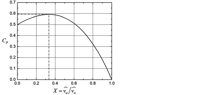
Figure 5. The Betz-Joukowsky limit. The solid line represents Equation (3.17) and the dash-dotted lines characterize the maximum of the power efficiency (with respect to Betz [58] ).
 . (3.18)
According to Betz [3] , and Joukowsky [4] , this value is the maximum wind power efficiency (see also [6] [11] [40] [58] [62] - [64] ).
Sometimes, the axial interference factor, a, defined by (e.g., [6] [11] [12] [62] [63] )
 , (3.19)
is inserted. Using this factor leads to
 (3.20)
and
 (3.21)
with . The axial interference factor measures the impact of the wind turbine on the air flow. In accord with the definition of this factor, the wind power efficiency and the thrust force can be expressed by
 (3.22)
and
 . (3.23)
The latter may be used to define the thrust coefficient,  , by (e.g., [6] [11] )
 . (3.24)
Thus, we have .
.
3.2. General Momentum Theory
The result of the Betz-Jowkowsky limit is based on simplified description of the flow field. Even though the flow field exhibits a pure axial behavior in front of the rotor, the exertion of a torque on the rotor disk by the air passing through it causes an equal, but opposite torque to be imposed on the air. Because of this reaction torque, the air starts to rotate in a direction opposite to that of the rotor; the air gains angular momentum and so in the wake of the rotor disk the air particles have a velocity component in a direction which is tangential to the rotation as well as having an axial velocity component [65] . Since the stream tube is opening behind the propeller, there is also a velocity component in the radial direction. Thus, by interacting with the rotor also velocity components in radial and azimuthal directions occur. The velocity vector at the rotor may be expressed by cylindrical polar co-ordinates; the velocity vector in the wake behind the rotor may be expressed in a similar manner.
To consider these rotational effects, Glauert [10] developed a simple model for the optimum rotor. In his approach, the rotor is a rotating axisymmetric actuator disk, corresponding to a rotor with an infinite number of blades [6] [11] [12] .
As outlined in Appendix B, the general equations of the General Momentum Theory lead to (see Equation (B.24))
 , (3.25)
where  is, again, the undisturbed wind speed far upstream of the wind turbine,
  is the angular velocity of the rotor,
  is the axial velocity through the propeller disk,
  is the angular velocity imparted to the slipstream,
  the axial velocity in the final wake, and
  the corresponding angular velocity at radial distance
 from the axis of the slipstream. Equation (3.25) already derived by Glauert [10] for an engine-driven propeller and by Wilson and Lissaman [62] for propeller-type wind turbines suffice to determine the relationship between the thrust and torque of the propeller and the flow in the slipstream. Owing to the complexity of the equations, however, it is customary to adopt certain approximations based on the fact that the rotational velocity in the slipstream is generally very small.
3.2.1. Joukowsky’s Constant Circulation Model
An exact solution of the general equations of the General Momentum Theory can be obtained when the flow in the slipstream is irrotational except along the axis [10] . This condition implies that the rotational momentum  has the same value k for all radial elements, i.e.,
 . (3.26)
Here, r is the radial distance of any annular element of the propeller disk. Equation (3.26) is the basis for Joukowsky’s constant circulation model [10] [65] .
On the basis of Equation (B.19) of Appendix B,
 , (3.27)
we can deduce that the axial velocity  is constant across the wake because
  and, hence,
 . Furthermore, Equation (3.25) is satisfied by a constant value of the axial velocity
  across the propeller disk. If
  and
and  are constant, we will obtain from the equation of continuity (see Equation (B.1)
of Appendix B),
 , (3.28)
and the conservation of angular momentum (see Equation (B.6) of Appendix B),
 , (3.29)
the following relationship [10]
 . (3.30)
In accord with Equation (3.30), Equation (3.25) becomes
 . (3.31)
If we assume again that , we will obtain (see Equation (B.14) of Appendix B)
 . (3.32)
Using the definitions  and
and  yields (see Equations (C.10) and (C.20) of Appendix C)
 (3.33)
and
 , (3.34)
where
 (3.35)
is the tip speed ratio. Thus,  , i.e., Equation (3.11) is not generally valid. Formula (3.34) was
already derived by Wilson and Lissaman [62] for a propeller-type wind turbine; a similar formula was given by Glauert [10] for an engine-driven propeller. Obviously, Equation (3.34) can only be solved iteratively. Results of such a solution are shown in Figure 6. As illustrated, for tip speed ratios in the range of , the axial interference factor, a, becomes negative. These results have to be discarded because they disagree with observations. For tip speed ratios
 , the condition
 , derived in the matter of the axial momentum theory, is nearly fulfilled [10] [62] . From Equation (3.34) we can infer that the condition
  is exactly fulfilled if
  becomes infinite.
In accord with Equation (2.54), the torque,  , experienced by this annular stream tube element between r and
  reads
reads
 , (3.36)
where the area of the stream tube element is , and k is given by Equation (3.26). Since the power caused by the rotor is the product of the angular velocity and this annulus torque, i.e.,
  , the integration over the total blade span provides
 . (3.37)
Replacing  with the aid of Equation (3.33) yields
 . (3.38)
Thus, in contrast to the axial momentum theory, the wind power efficiency is given by [60] [62]
 . (3.39)


Figure 6. Effect of the tip speed ratio l, defined by Equation (3.35), on the induced velocities for flow with an irrotational wake. The diagram on the right side is based on Figure 3.3 of Wilson and Lissaman [62] .
Inserting  into this formula provides Equation (3.22). This means that the power efficiency for the irrotational wake tends to that for the axial momentum theory (see Equation (3.22)) if the tip speed ratio exceeds
  [62] [65] . Since the ratio
  varies with
  (Figure 6), different tip speed ratios provide different curves for the power efficiency. The maximum power efficiency that is close to the Betz-Joukowsky limit of
0.593 occurs around  if the tip speed ratio exceeds
  (cf. Figure 7). Thus, for
we obtain . This is the value for which the Betz-Joukowsky limit was determined (see Figure 5 and Figure 7). Consequently, in case of an irrotational wake, the axial momentum theory provides reasonable results for tip speed ratios larger than
 .
.
Glauert [10] already argued:
The condition of constant circulation k along the blade, which has been the basis of the preceding calculations, cannot be fully realized in practice since it implies that near the roots of the blades the angular velocity imparted to the air is greater than the angular velocity of the propeller itself. In any practical application of the analysis it is therefore necessary to assume that the effective part of the propeller blades commences at a radial
distance not less than  at which
  is equal to
 .
.
It implies that, near the roots of the blades, the angular velocity imparted to the air is greater than the angular velocity of the propeller itself [6] . Wilson & Lissaman [62] and de Vries [40] shared Glauert’s viewpoint that the solution is unphysical as it results in infinite values of power and circulation when the tip-speed ratio tends to zero.
From Equations (3.30) and (3.33) we can derive
 (3.40)
or
 . (3.41)
The maximum values of the power efficiency for various tip speed ratios are also illustrated in Figure 8. This diagram shows that for  the maximum power efficiency notably exceeds the Betz-Joukowsky limit. However, these results must be assessed with care. For
 , for instance, we obtain
  that occurs at
 . According to Figure 6, for
  the axial interference factor amounts to
 . Consequently,
 and
and . These results seem to be unlikely because
  would only

Figure 7. Effect of the tip speed ratio l, defined by Equation (3.35), on the power efficiency for a flow with an irrotational wake.

Figure 8. Maximum power efficiency, CP,max, taken from Figure 7 versus tip speed ratio l defined by Equation (3.35).
be adequate in case of no wind turbine and  would require, in accord with Equation (3.30), that the
radius of the wake,  , must tend to infinity.
3.2.2. Glauert’s Optimum Rotor
For wind turbines, Glauert [10] derived an approximate solution on the basis of Equation (3.25). The angular velocity  imparted to the slipstream is, in general, very small compared with the angular velocity
  of the rotor. Therefore, it is possible to simplify the general equations by neglecting certain terms involving
 . Because of this simplification the pressure
  in the wake becomes equal to the initial pressure
  of the fluid, and the decrease of static pressure across the propeller disk is equal to the decrease of total pressure head, i.e.,
 . The relationships connecting the thrust and axial velocity are then the same as in the
simple axial momentum theory, the axial velocity  at the propeller disk is the arithmetic mean of the axial velocity
  and the slipstream velocity
 . Thus, in accord with Equation (B.20) of Appendix B, the element
of thrust becomes
 . (3.42)
Now, the torque experienced by this annular stream tube element is given by
 . (3.43)
Inserting ,
,  and
and  into these equation yields [10]
 (3.44)
and
 . (3.45)
Since the related power is given by , the integration over the total blade span provides [10] [62]
 . (3.46)
Defining  leads to
 . (3.47)
Thus, the power efficiency is given by [10] [62]
 . (3.48)
Alternatively, defining  provides [6] [56]
 . (3.49)
This formula is equivalent to Equation (3.48). Obviously, the power efficiency strongly depends the tip-speed ratio, but weighted by the integral expression. Unfortunately, Equations (3.48) and (3.49) contain the two unknowns a and . Thus, we need additional information for determining
 .
.
The pressure increment at the propeller disk is given by [62]
 . (3.50)
From Equations (3.44) and (3.50) we obtain
 . (3.51)
To obtain the maximum power for a given tip-speed ratio , the factors a and
  must be related by [10]
 (3.52)
and
 . (3.53)
Thus, combining Equations (3.51) to (3.53) provides
 (3.54)
and
 . (3.55)
The quantities ,
,  , and
, and  as a function of a are illustrated in Figure 9. In case of
 , we have a large value of
 , while the azimuthal interference factor,
  , is very small. The opposite is true in the case of
 . The quantities
  and
and  amount to
  and
and , respectively. Inserting these values of the interference factors into Equation (3.48) provides the power efficiency of the wind turbine. The relationship between
  and the tip-speed ratio
  is illustrated in Figure 10. Obviously, the maximum power efficiency depends on the tip-speed ratio. It approaches the Betz-Joukowsky limit at large tip- speed ratio only [6] [11] [62] .
3.3. Finite-Bladed Rotor Models
In case of finite-bladed rotor Equations (3.42) and (3.43) are imprecise. Based on the vortex theory, each of the rotor blades has to be replaced by a lifting line on which the radial distribution of bound vorticity is represented

Figure 9. The quantities ,
,  , and
, and  versus the axial interference factor
 .
.
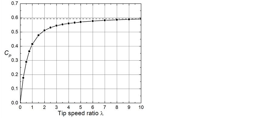
Figure 10. Power coefficient, CP, vs. tip-speed ratio, λ for Glauert’s [10] optimum actuator disk.
by the circulation  depending on the radial distance along the blade [11] [12] . This results in a free vortex system consisting of helical trailing vortices, as sketched in Figure 11. With respect to the vortex theory, the bound vorticity serves to produce the local lift on the blades while the trailing vortices induce the velocity field in the rotor plane and the wake [11] [12] . The velocity vector in the rotor plane is made up by the rotor angular velocity,
  , the undisturbed wind speed,
  , the axial and circumferential velocity components,
  , and
, and , respectively. These velocity components induced at a blade element in the rotor plane by the tip vortices (see Figure 12). Another circumferential velocity,
  is induced by the hub vortex (see Figure 12). To determine the velocity field given by
 ,
,  , and
, and  induced at a blade element in the rotor plane, the free half-infinite helical vortex system behind the rotor is replaced by ‘an associated vortex system’ that extends to infinity in both directions [12] . Neglecting deformations or changes in the wake, the vortex system is uniquely described by the far wake properties in the Trefftz plane [66] . It is defined as the plane normal to the relative wind far downstream of the rotor. In accordance with Helmholtz’ vortex theorem, the bound circulation
  around a blade element is uniquely related to the circulation of a corresponding vortex in the Trefftz plane [12] . By symmetry, the induced velocities at a point in the rotor plane equals half the induced velocity at a corresponding point in the Trefftz plane [67] -[70] , i.e.,
  ,
,  , and
, and  (see also [12] ).
Okulov and Sørensen [12] distinguished between two different concepts that dominated the conceptual interpretation of the optimum rotor: (a) Joukowsky [67] defined the optimum rotor as one having constant circulation along the blades, such that the vortex system for an  -bladed rotor consists of
  helical tip vortices of strength
  and an axial hub vortex of strength
 . A simplified model of this vortex system can be obtained by representing it as a rotating horseshoe vortex (Figure 11(a)). Betz and Prandtl [71] argued that optimum
 (a) (b)
Figure 11. Sketch of the vortex system corresponding to lifting line theory of the ideal propeller of (a) Joukowsky and (b) Betz (from Okulov and Sørensen [12] , but with respect to Sørensen [6] ).
 (a) (b)
Figure 12. Velocity and power triangles in the rotor plane of (a) Joukowsky rotor and (b) Betz rotor (adopted from Okulov and Sørensen [12] , but some symbols have changed to fit the text).
efficiency is obtained when the distribution of circulation along the blades generates a rigidly helicoidal wake that moves in the direction of its axis with a constant velocity. Betz used a vortex model of the rotating blades based on the lifting-line technique of Prandtl in which the vortex strength varies along the wing-span (Figure 11(b)). This distribution, usually referred to as the Goldstein circulation function, is rather complex and difficult to determine accurately [12] [72] .
Using the Kutta-Joukowsky-theorem
 , (3.56)
where  is the lift force on a blade element of radial dimension
 ,
,  is the resultant relative velocity and
  is the bound circulation, Okulov and Sørensen [11] deduced the local thrust and the local torque of a rotor blade given by
 (3.57)
and
 . (3.58)
Here, we only discuss the torque. Since the related power is given by , the integration over the total blade span provides for
  blades yields
 . (3.59)
Using the analytical solution to the induction of helical vortex filaments developed by Okulov [73] , Okulov & Sørensen [11] extended Goldstein’s [72] original formulation by a simple modification to handle heavily loaded rotors in accord with the general momentum theory. Assuming that the induction in the rotor plane equals half the induction in the Trefftz plane in the far wake, as described before, they found for the power efficiency
 . (3.60)
Here,  is the dimensionless translational velocity of the vortex sheet (see Figure 11(b))
 (3.61)
and
 , (3.62)
where  is the Goldstein [72] circulation function,
  ,
,  ,
,  is the pitch of the vortex sheet, and
  is the angle between the vortex sheet and the rotor plane. Thus, l may be expressed by
 . The first derivative test yields
 . (3.63)
The result of the second derivative test shows that Equation (3.63) characterizes the maximum of . As pointed out by Okulov and Sørensen [11] , for a rotor with infinitely many blades, both functions,
  and
and , tend to unity when the pitch tends to zero. In this case, Equation (3.60) degenerates to the expression
 . This result is completely consistent with the axial momentum theory because
  leads to Equation (3.22). Furthermore, Equation (3.63) provides
  and, hence,
 . This result is in
agreement with  that designates the maximum of
  in Figure 5.
In the vortex theory of the Joukowsky rotor [67] -[70] , each of the blades is replaced by a lifting line about which the circulation associated with the bound vorticity is constant, resulting in a free vortex system consisting of helical vortices trailing from the tips of the blades and a rectilinear hub vortex [12] . As sketched in Figure 11(a), the vortex system may be interpreted as consisting of rotating horseshoe vortices with cores of finite size, where the radius of the core is . The “associated vortex system” consists of a multiplet of helical tip vortices of finite vortex cores (
 ) with constant pitch h and circulation
 . The multiplet moves downwind (in case of a propeller) or upwind (in case of a wind turbine) with a constant velocity
  in the axial direction, where
  is the difference between the wind speed and axial translational velocity of the vortices [12] . Using the analytical solution to the induction of helical vortex filaments developed by Okulov [73] again, Okulov & Sørensen [12] derived for the power efficiency
 (3.64)
where  and
and
 . (3.65)
Here,  is the non-dimensional radius of the vortex core, and
  is a non-dimensional axial velocity. For a given helicoidal wake structure, the power coefficient is seen to be uniquely determined, except for the parameter a. The first derivative test yields
 . (3.66)
The result of the second derivative test shows that for this value of a characterizes the maximum of the power efficiency.
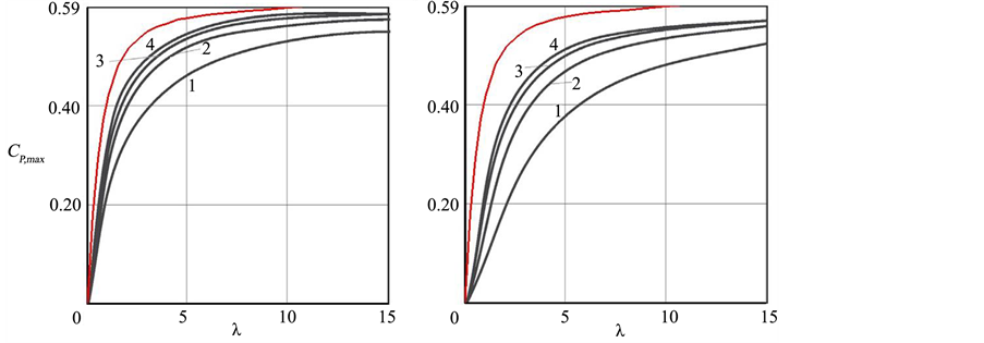
Figure 13 illustrates that the power coefficient computed by Okulov and Sørensen [11] [12] for various number of blades depends on the tip-speed ratio  given by Equation (3.35). Also shown is the result provided by Glauert’s [10] optimum actuator disk. Obviously, the optimum power coefficient of the Joukowsky rotor for all number of blades is larger than that for the Betz rotor, but the efficiency of the Betz rotor is larger if we compare it for the same deceleration of the wind speed [12] . The difference, however, vanishes for
  or for
 , where in both models tend towards the Betz-Joukowsky limit [12] .
Since neither the axial interference factor a nor  explicitly occurs in Equations (3.60) and (3.63),
  and a have to be connected to the helical pitch l and the generic parameter w by [12]
 (3.67)
and
 (a) (b)
Figure 13. Power coefficients, CP, of an optimum rotor as a function of tip speed ratio and number of blades. (a) Joukowsky rotor and (b) Betz rotor (adopted from Okulov and Sørensen [12] ). The red lines are added. They illustrate the solution of Glauert’s optimum actuator disk shown in Figure 10.
 , (3.68)
In case of the Joukowsky rotor the tip-speed ratio can be expressed by [12]
 . (3.69)
3.4. The Efficiency of Real Wind Turbines
Figure 14 shows the power curves of seven wind turbines of different rated power listed in Table 1. The power curves were determined by considering the listed values (only the Enercon machines) or by taking discrete values from the power curves illustrated in the actual brochures found at the manufacturers’ websites. Based on these discrete values, the parameters A, K, Q, B, M, and u of the generalized logistic function (e.g., [56] )
 . (3.70)
were numerically determined for each of the seven wind turbines (see Table 2). The function  represents the power generated by the corresponding wind turbine at the wind speed v.
Figure 15 illustrates the wind power density,  , for (a) a flow far upstream to the wind turbine given Equation (2.25) with
 , (b) an “ideal” wind turbine generating wind power by obeying the Betz-

Figure 14. Wind power density of seven wind turbines of different rated power considered in this study. They are based on the parameters of the generalized logistic function (see Equation (3.70)) listed in Table 2.

Table 1. Specifications of the wind turbines considered in this study.

Figure 15. Wind power densities of the seven wind turbines listed in Table 1. Also shown are the wind power density  given by Equation (2.25), and
  weighted by the Betz-Joukowsky limit.
Table 2. Parameters A, K, Q, B, M, and u of the generalized logistic function (3.70) used to model the wind turbines’ power curves.
Joukowsky limit of , and (c) the power curves of the seven wind turbines shown in Figure 14, but normalized by the corresponding swept areas. As shown in Figure 15, the wind power densities are lower than the Betz-Joukowsky limit, but follow it up to a wind speed at hub height of
  or so. Beyond this wind speed, they approach plateau values at the rated wind speeds; these plateau values are ranging from
  (General Electric 1.6-82.5) to
  (Enercon E-82 E4). The two other wind power densities continuously increase because of the
  -law. Thus, the power efficiencies of all wind turbines considered here are notably higher than the 30-percent limit of Gorban’ et al. [1] for wind speeds between
  and
and  (see Figure 16). In case of wind speeds higher than
 , the power efficiencies eventually fall below this 30-percent limit and approach very low values in the vicinity of the cut-out wind speed.
4. Summary and Conclusions
We demonstrated that the filtration equation used by Gorban’ et al. [1] for determining the maximum efficiency of plane propellers at about 30 percent for free fluids plays no role in describing the flows in the ABL and has to be discarded. The ABL is mainly governed by turbulent motion, even though the effect of the turbulence intensity

Figure 16. Power efficiencies of the seven wind turbines listed in Table 1 (in accord with Enercon’s product overview updated in September 2012).
is relatively small in the undisturbed wind field over water surfaces. This effect may become more influential in case of aerodynamically rougher landscapes covered, for instance, with vegetation canopies. In case of wind farms the effect by turbulence may considerably increase inside the array of wind turbines. Based on Equation (2.57), we showed that the criticism of van Kuik et al. [9] regarding the work of Gorban’ et al. [1] is quite justified.
We also demonstrate that the stream tube model customarily applied to derive the Rankine-Froude theorem must be corrected in the sense of Glauert to provide an appropriate value for the axial velocity at the rotor area. Including this correction leads to the Betz-Joukowsky limit, namely of a maximum efficiency of 59.3 percent.
We also assessed Joukowsky’s constant circulation model that leads to values of the maximum efficiency exceeding the Betz-Jowkowsky limit for very low tip speed ratios. Some of these values, however, have to be rejected because of physical reasons.
Using Glauert’s [10] optimum actuator disk, and the results of the blade-element analysis by Okulov and Sørensen [11] [12] we illustrated that the maximum efficiency of propeller-type wind turbines depends on tip- speed ratio and the number of blades.
Finally, we showed that the power efficiencies of seven wind turbines of different rated power are notably higher than 30-percent limit of Gorban’ et al. [1] for wind speeds between  and
and . In case of wind speeds higher than
 , the power efficiencies eventually fall below this 30-percent limit and approach very low values in the vicinity of the cut-out wind speed.
Acknowledgements
We would like to express much gratitude to the Alaska Department of Labor for funding Dr. Gary Sellhorst’s project work. We would like to extend gratitude to the National Science Foundation for funding the project work of Hannah K. Ross and John Cooney in summer 2012 through the Research Experience for Undergraduates (REU) Program, grant number AGS1005265. We also express our thanks to the Max Planck Institute for Chemistry for the current financial support for Dr. Dr. habil. Ralph Dlugi.
Cite this paper
GerhardKramm,GarySellhorst,Hannah K.Ross,JohnCooney,RalphDlugi,NicoleMölders, (2016) On the Maximum of Wind Power Efficiency. Journal of Power and Energy Engineering,04,1-39. doi: 10.4236/jpee.2016.41001
References
- 1. Gorban’, A.N., Gorlov, A.M. and Silantyev, V.M. (2001) Limits of the Turbine Efficiency for Free Fluid Flow. Journal of Energy Resources Technology, 123, 311-317.
http://dx.doi.org/10.1115/1.1414137 - 2. Okulov, V.L. and van Kuik, G.A.M. (2011) The Betz-Joukowsky Limit: On the Contribution to Rotor Aerodynamics by the British, German and Russian Scientific Schools. Wind Energy, 15, 355-344.
http://dx.doi.org/10.1002/we.464 - 3. Betz, A. (1920) Das Maximum der theoretisch möglichen Ausnützung des Windes durch Windmotoren. Zeitschrift für das gesamte Turbinenwesen, 26, 307-309. (In German)
- 4. Joukowsky, N.E. (1920) Windmill of the NEJ Type. Transactions of the Central Institute for Aero-Hydrodynamics of Moscow. (In Russian) (as cited by )
- 5. van Kuik, G.A.M. (2007) The Lanchester-Betz-Joukowsky Limit. Wind Energy, 10, 289-291.
http://dx.doi.org/10.1002/we.218 - 6. Sørensen, J.N. (2011) Aerodynamic Aspects of Wind Energy Conversion. Annual Review of Fluid Mechanics, 43, 427-448.
http://dx.doi.org/10.1146/annurev-fluid-122109-160801 - 7. Hartwanger, D. and Horvat, A. (2008) 3D Modelling of Wind Turbine Using CFD. NAFEMS UK Conference 2008 “Engineering Simulation: Effective Use and Best Practice”, Cheltenham, 10-11 June 2008, 14 p.
- 8. Blackledge, J., Coyle, E. and Kearney, D. (2011) A Stochastic Model for Wind Turbine Power Quality Using a Levy Index Analysis of Wind Velocity Data. The Third International Conference on Resource Intensive Applications and Services, Venice, 22-27 May 2011.
- 9. van Kuik, G.A.M., Sørensen, J.N. and Okulov, V.L. (2015) Rotor Theories by Professor Joukowsky: Momentum Theories. Progress in Aerospace Sciences, 73, 1-18.
http://dx.doi.org/10.1016/j.paerosci.2014.10.001 - 10. Glauert, H. (1935) Airplane Propellers. In: Durand, W.F., Ed., Aerodynamic Theory, Vol. IV, Division L, Springer, New York, 169-360.
http://dx.doi.org/10.1007/978-3-642-91487-4_3 - 11. Okulov, V.L. and Sørensen, J.N. (2008) Refined Betz Limit for Rotors with a Finite Number of Blades. Wind Energy, 11, 415-426.
http://dx.doi.org/10.1002/we.274 - 12. Okulov, V.L. and Sørensen, J.N. (2010) Maximum Efficiency of Wind Turbine Rotors Using Joukowsky and Betz Approaches. Journal of Fluid Mechanics, 649, 497-508.
http://dx.doi.org/10.1017/S0022112010000509 - 13. de Groot, S.R. and Mazur, P. (1969) Non-Equilibrium Thermodynamics. North-Holland Publishing Comp., Amsterdam/ London.
- 14. Landau, L.D. and Lifschitz, E.M. (1981) Lehrbuch der theoretischen Physik-Hydrodynamik. Akademie-Verlag Berlin. (In German)
- 15. Budó, A. (1990) Theoretische Mechanik. In: Rompe, R. and Schmutzer, E., Eds., Hochschulbücher für Physik, VEB Deutscher Verlag der Wissenschaften, Berlin, 615. (In German)
- 16. Mölders, N. and Kramm, G. (2014) Lectures in Meteorology. Springer International Publishing.
http://dx.doi.org/10.1007/978-3-319-02144-7 - 17. Prandtl, L. (1905) über Flüssigkeitsbewegung bei sehr kleiner Reibung. Verhandlungen des III. Internationalen Mathematiker Kongresses, Heidelberg, 8-13 August 1904, B. G. Teubner, Leipzig, 485-491. (In German)
- 18. Rotta, J.C. (1972) Turbulente Strömungen. B. G. Teubner, Stuttgart. (In German)
http://dx.doi.org/10.1007/978-3-322-91206-0 - 19. Sanderse, B., van der Pijl, S.P. and Koren, B. (2011) Review of Computational Fluid Dynamics for Wind Turbine Wake Aerodynamics. Wind Energy, 14, 799-819.
http://dx.doi.org/10.1002/we.458 - 20. Reynolds, O. (1895) On the Dynamical Theory of Incompressible Viscous Fluids and the Determination of the Criterion. Philosophical Transactions of the Royal Society of London, 186, 123-164.
http://dx.doi.org/10.1098/rsta.1895.0004 - 21. Prandtl, L. (1918) Tragflügeltheorie—I. Mitteilung. Nachrichten der K. Gesellschaft zu Göttingen, Mathematisch-Physikalische Klasse, 451-477.
- 22. Kramm, G. and Meixner, F.X. (2000) On the Dispersion of Trace Species in the Atmospheric Boundary Layer: A Re-formulation of the Governing Equations for the Turbulent Flow of the Compressible Atmosphere. Tellus, 52A, 500-522.
http://dx.doi.org/10.1034/j.1600-0870.2000.00984.x - 23. Montgomery, R.B. (1954) Convection of Heat. Archiv für Meteorologie,Geophysik und Bioklimatologie, A7, 125-132.
http://dx.doi.org/10.1007/BF02277911 - 24. Fortak, H. (1969) Zur Energetik der planetarischen Grenzschicht. Annalen der Meteorologie (NF) 4, 157-162. (In German)
- 25. van Mieghem, J. (1949) Les equations générales de la mécanique et de l'énergétique des milieux turbulents en vue des applications à la météorologie. Inst. R. Météor. Belgique., Mém., XXXIV, 60. (In French)
- 26. van Mieghem, J. (1973)Atmospheric Energetics. Clarendon Press, Oxford, UK.
- 27. Herbert, F. (1975) Irreversible Prozesse der Atmosphäre—3. Teil (Phänomenologische Theorie mikroturbulenter Systeme). Beiträge zur Physik der Atmosphäre, 48, 1-29. (In German)
- 28. Libby, P.A. and Williams, F.A., Eds. (1980) Turbulent Reacting Flows. Springer-Verlag, Berlin.
http://dx.doi.org/10.1007/3-540-10192-6 - 29. Pichler, H. (1984) Dynamic der Atmosphäre. Bibliographisches Institut, Zürich. (In German)
- 30. Cox, G. (1995) Basic considerations. In: Cox, G., Ed., Combustion Fundamentals of Fire, Academic Press, London, San Diego, New York, 3-30.
- 31. Kramm, G., Dlugi, R. and Lenschow, D.H. (1995) A Re-evaluation of the Webb-Correction Using Density-Weighted Averages. Journal of Hydrology, 166, 283-292.
http://dx.doi.org/10.1016/0022-1694(94)05088-F - 32. Thomson, D. (1995) The Parameterization of the Vertical Dispersion of a Scalar in the Atmospheric Boundary Layer. Atmospheric Environment, 29, 1343.
http://dx.doi.org/10.1016/1352-2310(94)00326-G - 33. Venkatram, A. (1998) Response. Atmospheric Environment, 32, 259.
http://dx.doi.org/10.1016/S1352-2310(96)00078-7 - 34. Kowalski, A.S. (2012) Exact Averaging of Atmospheric State and Flow Variables. Journal of the Atmospheric Sciences, 69, 1750-1757.
http://dx.doi.org/10.1175/JAS-D-11-0299.1 - 35. Hesselberg, T. (1926) Die Gesetze der ausgeglichenen atmosphärischen Bewegungen. Beiträge zur Physik der freien Atmosphäre, 12, 141-160. (In German)
- 36. Lumley, J.L. and Yaglom, A.M. (2001) A Century of Turbulence. Flow, Turbulence and Combustion, 66, 241-286.
http://dx.doi.org/10.1023/A:1012437421667 - 37. Herbert, F. (1995) A Re-evaluation of the Webb Correction Using Density-Weighted Averages—Comment. Journal of Hydrology, 173, 343-344.
http://dx.doi.org/10.1016/0022-1694(95)02867-o - 38. Eliassen, A. and Kleinschmidt Jr., E. (1957) Dynamic Meteorology. In: Flügge, S., Ed., Handbuch der Physik, Bd. XLVIII. Springer-Verlag Berlin/Heidelberg/New York, 1-154.
http://dx.doi.org/10.1007/978-3-642-45881-1_1 - 39. Dutton, J.A. (1995) Dynamics of Atmospheric Motion. Dover, New York.
- 40. de Vries, O. (1979) Fluid Dynamic Aspects of Wind Energy Conversion. AGARDograph 243, AGARD, Brussels.
- 41. Türk, M. and Emeis, S. (2010) The Dependence of Offshore Turbulence Intensity on Wind Speed. Journal of Wind Engineering and Industrial Aerodynamics, 98, 466-471.
http://dx.doi.org/10.1016/j.jweia.2010.02.005 - 42. Barthelmie, R.J., Frandsen, S.T., Nielsen, M.N., Pryor, S.C., Rethore, P.-E. and Jørgensen, H.E. (2007) Modelling and Measurements of Power Losses and Turbulence Intensity in Wind Turbine Wakes at Middelgrunden Offshore Wind Farm. Wind Energy, 10, 517-528.
http://dx.doi.org/10.1002/we.238 - 43. Barthelmie, R.J., Churchfield, M.J., Moriarty, P.J., Lundquist, J.K., Oxley, G.S., Hahn, S. and Pryor, S.C. (2015) The Role of Atmospheric Stability/Turbulence on Wakes at the Egmond aan Zee Offshore Wind Farm. Journal of Physics: Conference Series, 625, conference 1.
http://dx.doi.org/10.1088/1742-6596/625/1/012002 - 44. Stull, R.B. (1988) An Introduction to Boundary Layer Meteorology. Kluwer Academic Publishers, Dordrecht, Boston, London.
http://dx.doi.org/10.1007/978-94-009-3027-8 - 45. Garratt, J.R. (1994) The Atmospheric Boundary Layer. Cambridge University Press, Cambridge, New York, Melbourne.
- 46. Mellor, G.L. and Yamada, T. (1974) A Hierarchy of Turbulence Closure Models for Planetary Boundary Layers. Journal of the Atmospheric Sciences, 31, 1791-1806.
http://dx.doi.org/10.1175/1520-0469(1974)031<1791:AHOTCM>2.0.CO;2 - 47. Mellor, G.L. and Yamada, T. (1982) Development of a Turbulence Closure Model for Geophysical Fluid Problems. Review of Geophysics and Space Physics, 20, 851-875.
http://dx.doi.org/10.1029/RG020i004p00851 - 48. Janjic, Z.I. (2001) Nonsingular Implementation of the Mellor-Yamada Level 2.5 Scheme in the NCEP Meso Model. National Centers for Environmental Prediction (NCEP), Office Note #437.
- 49. Lorenz, E.N. (1967) The Nature and Theory of the General Circulation of the Atmosphere. World Meteorological Organization, WMO-No. 218.Tp.115, Geneva.
- 50. Bernhardt, K. and Lauter, E.A. (1977) Globale physikalische Prozesse und Umwelt. Zeitschrift für Meteorologie, 27, 1-20. (In German)
- 51. Holton, J.R. (1979) An Introduction to Dynamic Meteorology. Academic Press, New York, San Francisco, London.
- 52. Peixoto, J.P. and Oort, A.H. (1992) Physics of Climate. Springer-Verlag, New York, Berlin, Heidelberg.
- 53. Hilbert, D. and Cohn-Vossen, S. (1952) Geometry and the Imagination. Chelsea Publishing Company, New York.
- 54. Lass, H. (1950) Vector and Tensor Analysis. McGraw-Hill, New York, Toronto, London.
- 55. Alekseenko, S.V., Kuibin, P.A. and Okulov, V.L. (2007) Theory of Concentrated Vortices. Springer, Berlin, Heidelberg, New York.
- 56. Ross, H.K., Cooney, J., Hinzman, M., Smock, S., Sellhorst, G., Dlugi, R, Mölders, N. and Kramm, G. (2014) Wind Power Potential in Interior Alaska from a Micrometeorological Perspective. Atmospheric and Climate Sciences, 4, 100-121.
http://dx.doi.org/10.4236/acs.2014.41013 - 57. Goorjian, P.M. (1972) An Invalid Equation in the General Momentum Theory of the Actuator Disc. AIAA Journal, 10, 543-544.
http://dx.doi.org/10.2514/3.50146 - 58. Betz, A. (1926) Wind-Energie und Ihre Ausnutzung durch Windmühlen. Vandenhoeck & Ruprecht, Göttingen, Germany. (In German)
- 59. Rankine, W.J.M. (1865) On the Mechanical Principles of the Action of Propellers. Transaction of the Institute of Naval Architects, 6, 13-39.
- 60. Froude, W. (1878) On the Elementary Relation between Pitch, Slip and Propulsive Efficiency. Transaction of the Institute of Naval Architects, 19, 22-33.
- 61. Froude, R.E. (1889) On the Part Played in Propulsion by Difference in Pressure. Transaction of the Institute of Naval Architects, 30, 390-405.
- 62. Wilson, R.E. and Lissaman, P.B.S. (1974) Applied Aerodynamic Performance of Wind Power Machines. Oregon State University, Corvallis.
- 63. Snel, H. (1998) Review of the Present Status of Rotor Aerodynamics. Wind Energy, 1, 46-69.
http://dx.doi.org/10.1002/(SICI)1099-1824(199804)1:1+<46::AID-WE3>3.3.CO;2-0 - 64. Mathew, S. (2006) Wind Energy: Fundamentals, Resource Analysis, and Economics. Springer.
http://dx.doi.org/10.1007/3-540-30906-3 - 65. Sharpe, D. (2004) A General Momentum Theory Applied to an Energy-Extracting Actuator Disc. Wind Energy, 7, 177-188.
http://dx.doi.org/10.1002/we.118 - 66. Trefftz, E. (1921) Zur Prandtlschen Tragflächentheorie. Math. Ann., 82, 306-319.
http://dx.doi.org/10.1007/BF01498674 - 67. Joukowsky, N.E. (1912) Vortex Theory of Screw Propeller, I. Trudy Otdeleniya Fizicheskikh Nauk Obshchestva Lubitelei Estestvoznaniya 16 (1), 1-31 (In Russian). French translation in: Théorie tourbillonnaire de l’hélice propulsive (Gauthier-Villars, Paris, 1929) 1-47 (as cited by ).
- 68. Joukowsky, N.E. (1914) Vortex Theory of Screw Propeller, II. Trudy Otdeleniya Fizicheskikh Nauk Obshchestva Lubitelei Estestvoznaniya 17 (1), 1-33 (In Russian). French translation in: Théorie tourbillonnaire de l’hélice propulsive (Gauthier-Villars, Paris, 1929) 48-93 (as cited by ).
- 69. Joukowsky, N.E. (1915) Vortex Theory of Screw Propeller, III. Trudy Otdeleniya Fizicheskikh Nauk Obshchestva Lubitelei Estestvoznaniya 17 (2), 1-23 (In Russian). French translation in: Théorie tourbillonnaire de l’hélice propulsive (Gauthier-Villars, Paris, 1929) 94-122 (as cited by ).
- 70. Joukowsky, N.E. (1918) Vortex Theory of Screw Propeller, IV. Trudy Avia Raschetno-Ispytatelnogo Byuro, no 3, 1-97 (In Russian). French translation in: Théorie tourbillonnaire de l’hélice propulsive (Gauthier-Villars, Paris, 1929) 123-198 (as cited by ).
- 71. Betz, A. (1919) Schraubenpropeller mit geringstem Energieverlust—Mit einem Zusatz von L. Prandtl. Nachrichten d. K. Gesellschaft d. Wissenschaften, Göttingen, Math.-phys. Klasse, 193-217. (In German)
- 72. Goldstein, S. (1929) On the Vortex Theory of Screw Propellers. Proceedings of the Royal Society of London. Series A, 123, 440-465.
http://dx.doi.org/10.1098/rspa.1929.0078 - 73. Okulov, V.L. (2004) On the Stability of Multiple Helical Vortices. Journal of Fluid Mechanics, 521, 319-342.
http://dx.doi.org/10.1017/S0022112004001934 - 74. Haltiner, G.J. and Martin, F.L. (1957) Dynamical and Physical Meteorology. McGraw-Hill, New York, Toronto, London.
- 75. Thomas, T.Y. (1961) Concepts from Tensor Analysis and Differential Geometry. Academic Press, New York, London.
- 76. Sokolnikoff, I.S. (1964) Tensor Analysis: Theory and Applications to Geometry and Mechanics of Continua. 2nd Edition, John Wiley & Sons, New York, London, Sydney.
- 77. Eisenreich, G. (1971) Vorlesungen über Vektorund Tensorrechnung. BSB B.G. Teubner Verlagsgesellschaft, Leipzig. (In German)
- 78. Teichmann, H. (1973) Physikalische Anwendungen der Vektor-und Tensorrechnung. Bibliographisches Institut Mannheim, Wien, Zürich. (In German)
- 79. Fortak, H. (1967) Vorlesungen über theoretische Meteorologie-Kinematik der Atmosphäre. Freie Universität Berlin, Institut für Theoretische Meteorologie. (In German)
Appendix A: Trajectories versus Streamlines
Let us consider a natural coordinate frame with the unit vectors ,
,  , and
, and  that form a right-handed rectangular coordinate system at any given point of a curve in space (moving trihedron) like a trajectory (Figure 3), where the subscript t characterizes the trajectory-related quantities. Such a frame describing the movement of a particle along its trajectory in space is called an intrinsic system because it is closely related to the motion itself (e.g., [16] [54] [74] ). As illustrated in Figure 3, the unit vector
  is related to the direction of the instantaneous motion at any point, i.e., it is tangent to the curve of the trajectory, and is, therefore, called the unit tangent. The velocity vector is given by
 , where V is its magnitude. The moving trihedron consisting of
 ,
,  , and
, and  is an orthonormal frame, i.e., the orthonormal conditions
 (A.1)
(A.1)
and
 . (A.2)
are fulfilled. These unit vectors can be considered as either contravariant or covariant basis vectors. We may write
 . (A.3)
because the triple scalar product . The unit vector
  is the principal normal.
The unit vector  is perpendicular to the osculating plane spanned by
  and
and , and called the binormal. The plane containing
  and
and  is the normal plane, and the plane determined by
  and
and  is the rectifying plane (e.g., [53] ). As the unit tangent
  is time-dependent, the other two basis vectors depend on time, too. The unit tangent is defined by
 , (A.4)
where  is the position vector, and s is the arc length. From Equation (A.4) we can infer that
 . Thus, the arc length between two points
  and
and  is given by
 . (A.5)
The principal normal  is referred to the change of the unit vector
  along the space trajectory because
 . (A.6)
This means that  and
and  are perpendicular to each other, or in other words,
  is normal to the curve of the trajectory. The magnitude of
  is defined as the curvature
  of the trajectory at a given point. Thus, we have
 . (A.7)
We may also define a radius of curvature by . As
. As
 . (A.8)
and
 , (A.9)
we may infer that  is perpendicular to both
  and
and . Thus,
  can also be expressed by
 , (A.10)
where the proportionality constant  is the torsion. For the derivative of
  with respect to s we obtain
 . (A.11)
The relations (A.7), (A.10), and (A.11) can be summarized as follows
 . (A.12)
These equations are the central equations in the theory of space curves customarily called the Serret-Frenet formulae (e.g., [74] - [76] ). The Serret-Frenet formulae (A.12) allow to determine the change of the vectors of the trihedron,  ,
,  , and
, and , while it is moving along a given space curve
  as a function of the arc length s.
Equation (A.11) may also be written as
 . (A.13)
The vector  that lies in the rectifying plane (see Figure 3) is the Darboux vector of a space curve (e.g., [77] [78] ). Using this definition yields
 . (A.14)
Obviously, the Darboux vector determines the new orientation (rotation) of the moving trihedron (see Figure 3). In other words, the Darboux vector coincides with the instantaneous axis of rotation. If  denotes the instantaneous angular velocity vector and V the instantaneous speed, we will have
 . (A.15)
The magnitude of the Darboux vector is the total curvature, sometimes also called the Lancret curvature (e.g., [79] ).
A trajectory is the actual path of an air particle, i.e., it characterizes the direction of the velocity that such an air particle is taking successively during a certain time interval (e.g., [79] ). If the velocity field  is always known during that time interval, the trajectory can be calculated by integration of
 . A streamline represents a “snapshot” of the directions of the velocity field
  at various locations at time
 . As at each location a streamline is parallel to the flow field, we may write
 . (A.16)
As sketched in Figure 3, a trajectory is the envelope of the corresponding streamlines. Thus, at a certain point  the unit tangent
  represents both the direction of this trajectory and the direction of the streamline touching the trajectory at this certain point. Even though the unit tangent is the same, the principal normal,
  , and the binormal,
  , of the trajectory generally differ from the principal normal,
  , and the binormal,
  , of the streamline, i.e.,
  and
and . However, we have
 . (A.17)
If we express the substantial derivative of the unit tangent in the Eulerian form, we will obtain
 . (A.18)
Here, the partial derivative of the unit tangent with respect to the arc length was replaced by , where
  is the curvature of the streamline and
  is the corresponding radius of the curvature. On the
other hand, we have
 . (A.19)
Combining Equations (A.18) and (A.19) yields
 . (A.20)
In the two-dimensional case, we have  because
 . Thus, Equation (A.20) becomes
 . (A.21)
With respect to the unit vectors  and
and  of a Cartesian frame the unit tangent of a plane trajectory can be expressed by
 . (A.22)
where  is the angle between
  and
and . It is also the angle between
  and
and . This angle usually depends on time. Thus, the local rate of change of the unit tangent reads
 . (A.23)
Combining Equations (A.21) and (A.23) yields
 . (A.24)
The scalar form of the relation (A.24) is Blaton’s equation. In the case of steady-state conditions, the left-hand side terms of Equations (A.21) and (A.24) vanish and the curvatures of the trajectories and the streamlines are identical, i.e., the trajectories and the streamlines coincide.
If no tangential acceleration exists, i.e.,  , and the horizontal scale is small enough, so that the mag-
nitude of Coriolis acceleration is small in comparison with those of the centripetal acceleration and the acceleration due to the pressure gradient, we will lead to the following conditions for a frictionless flow:
 (A.25)
and
 . (A.26)
The solution of this equation set is then given by
 . (A.27)
The equation describes the cyclostrophic flow. Obviously,  and
and  must have opposite signs to ensure that the condition
 . (A.28)
is fulfilled. Both cyclonic and anti-cyclonic flows are possible. Assuming, for instance,  ,
,  , and
, and  yields
 . The cyclostrophic approximation is acceptable if the Ross by number defined by
 (A.29)
fulfills the condition . Figure 17 shows the wind speed V as a function of the pressure gradient
  in case of a cyclostrophic flow, where
  and
and  were assumed. As illustrated, even small values of the pressure gradient like
  can produce a cyclostrophic wind speed of more than
 . In such a case the Rossby number amounts to
  if a typical value of
  for the Coriolis parameter is considered. In case of
 ,
,  , and
, and , the Rossby number is
 . These numbers are typical for an F1 tornado on the Fujita Tornado Damage Scale. The occurrence of a cyclostrophic flow has to be considered if a difference between the static pressure far upstream and far downstream of a wind turbine is presupposed.
Appendix B: The Equations of the General Momentum Theory
In this appendix, we only consider average values. Thus, all symbols that are characterizing average values are ignored here. Let be r the radial distance of any annular element of the propeller disk,  and
and  the axial and the radial components of the fluid velocity, respectively. Furthermore, let be p the pressure immediately in front of the propeller and
  the decrease of the pressure behind the propeller associated with the angular velocity
 . Moreover, let
  be the pressure in the final wake,
  the corresponding axial velocity, and
  the corresponding angular velocity at radial distance
  from the axis of the slipstream. Since the area of the annular element is
 , the equation of continuity reads
 (B.1)
(B.1)
Generally, the torque is
 (B.2)
(B.2)
If the force  is only a function of the radial vector
  of the form
 , as considered here, we will obtain
 . Since the torque is equal to the derivative of the angular momentum,
  , with respect to time, we may write
 (B.3)
(B.3)
i.e., the angular momentum is invariant with time ( ). Equation (B.3) describes the conservation of angular momentum in the central field. The angular momentum can be expressed by

Figure 17. Wind speed versus pressure gradient in case of a cyclostrophic flow.
 (B.4)
(B.4)
where  is the velocity vector of a particle with the mass m moving through the central field. As
  and
and  throughout the motion, the radius vector of the particle on which the central field is acting lies in the plane spanned by
  and
and  which is perpendicular to
 . Hence, we may write for convenience
 (B.5)
(B.5)
Thus, the conservation of angular momentum provides
 . (B.6)
In accord with Equation (2.54), the torque is given by
 . (B.7)
The Bernoulli equation in its approximated form (2.46) yields
 . (B.8)
and
 . (B.9)
Thus, the difference of the total pressure heads,  , is given by
 . (B.10)
In addition, the pressure difference  reads
reads
 , (B.11)
where the conservation of the angular momentum (see Equation (B.6)) has been used. Rearranging  by
by

leads to
 . (B.12)
Here,  is the angular velocity of the rotor.
In applying Bernoulli's equation to the flow relative to the propeller blades, we have to consider the relative angular velocity of the air that increases from  to
to  associated with a decrease of the static pressure behind the propeller and given by
 . (B.13)
Thus, we obtain
 . (B.14)
The pressure gradient in the wake balances the centrifugal force on the fluid and is governed by
 . (B.15)
A balance between the pressure gradient force and the centrifugal force in the horizontal direction leads to the cyclostrophic flow well known in meteorology (e.g., [12] ). The derivation of Equation (B.14) with respect to  leads to
 (B.16)
or
 , (B.17)
where Equation (B.15) was used. Since
 , (B.18)
Equation (B.17) becomes [62]
 . (B.19)
Furthermore, the thrust is given by
 . (B.20)
The pressure increment at the propeller disk is given by [62]
 . (B.21)
Combining these two equations leads to
 . (B.22)
The equation of continuity provides  (see Equation (B.1)). Thus, we obtain
 . (B.23)
Finally, using  yields
 . (B.24)
This equation already derived by Wilson and Lissaman [62] suffice to determine the relationship between the thrust and torque of the propeller and the flow in the slipstream. Owing to the complexity of the equations, however, it is customary to adopt certain approximations based on the fact that the rotational velocity in the slipstream is generally very small.
Since Sharpe [65] criticized the work of Glauert [10] , Wilson and Lissaman [62] and others because of their dropping of the static pressure in the wake, we compared Sharpe’s equation (4), (7), (8), and (11) with our Equations (B.11), (B.13), (B.14), and (B.19). Rearranging Equation (B.11) yields
 . (B.25)
Using ,
,  ,
,  , and
, and  yields
  and
and , so that Equation (B.25) becomes
 . (B.26)
This is identical with Sharpe’s Equation (4). Considering  (see Equation (B.6)) leads to Sharpe’s Equation (5). In a similar manner, we obtain from Equation (B.13)
 . (B.27)
that is identical with Sharpe’s Equation (7). Thus, our Equation (B.14) results in
 . (B.28)
This equation completely agrees with Sharpe’s Equation (8). Finally, by rearranging our Equation (B.19)we obtain
 . (B.29)
that is identical with Sharpe’s Equation (11). Thus, Equation (B.24) already derived by Wilson and Lissaman [62] and the opposite one derived by Glauert [10] are accurate if an actuator disk is considered. Sharpe’s criticism is, therefore, not justified.
Appendix C: Solution of an Irrotational Wake
An exact solution of the general equations of the General Momentum Theory described before can be obtained when the flow in the slipstream is irrotational except along the axis [10] [65] . This condition implies that the rotational momentum  has the same value k for all radial elements, i.e.,
 . (C.1)
Here, r the radial distance of any annular element of the propeller disk.
On the basis of the equation (see Equation (B.19) of Appendix B)
 (C.2)
(C.2)
we can deduce that the axial velocity  is constant across the wake because
  and, hence,
 . Furthermore, it can be shown that Equation (B.24) of Appendix B is satisfied by a constant value of the axial velocity
  across the propeller disk. If
  and
and  are constant, we will obtain from the equation of continuity (see Equation (B.1) of Appendix B),
 , (C.3)
and the conservation of angular momentum (see Equation (B.6) of Appendix B),
 , (C.4)
the following relationship [10]
 (C.5)
(C.5)
or with respect to Sharpe’s [65] notation
 , (C.6)
where ,
,  , R is the radius of the rotor,
  is the maximum value of
 ,
,
 (C.7)
(C.7)
is the azimuthal interference factor, and by analogy with that quantity,
 , (C.8)
considered for the fully developed wake. Thus, Equation (B.24) of Appendix B becomes
 (C.9)
(C.9)
or
 . (C.10)
In accord with Glauert [10] , we define
 , (C.11)
 , (C.12)
 , (C.13)
and
 . (C.14)
Inserting these definitions into Equation (C.9) yields
 . (C.15)
If we assume again, that , we will obtain from Equation (B.14) of Appendix B
 (C.16)
or
 . (C.17)
Inserting Equation (C.11) into this equation provides
 . (C.18)
Rearranging this equation yields
 . (C.19)
Since  and
and , we obtain
 . (C.20)
This formula was already derived by Wilson and Lissaman [62] , but they used , where
  is, again, the tip speed ratio. A similar formula was also deduced by Glauert [10] for an engine-driven propeller.
NOTES

*Corresponding author.