ABSTRACT

Object classification in high-density 3D point clouds with applications in precision farming is a very challenging area due to high intra-class variances and high degrees of occlusions and overlaps due to self-similarities and densely packed plant organs, especially in ripe growing stages. Due to these application specific challenges, this contribution gives an experimental evaluation of the performance of local shape descriptors (namely Point-Feature Histogram (PFH), Fast-Point-Feature Histogram (FPFH), Signature of Histograms of Orientations (SHOT), Rotational Projection Statistics (RoPS) and Spin Images) in the classification of 3D points into different types of plant organs. We achieve very good results on four representative scans of a leave, a grape bunch, a grape branch and a flower of between 94 and 99% accuracy in the case of supervised classification with an SVM and between 88 and 96% accuracy using a k-means clustering approach. Additionally, different distance measures and the influence of the number of cluster centres are examined.

Keywords:

Descriptor Performance, Precision Farming, 3D Data

1. Introduction

The automatic analysis of 3D point clouds generated from plant data is an important step on the way to automatic phenotyping, where phenotypes refer to the observable attributes of a plant. Manual phenotyping is widely recognized to be labour-intensive and highly time-consuming, also known as the “phenotyping bottleneck” [1] . A lot of effort is poured into the automatization of this task.

3D scanners allow the generation of 3D data from plants in a non-invasive way, simply by moving the scanner around the object. Today, there are relatively cheap scanners providing a sufficient resolution to scan even fine stalks and being independent of the illumination, giving rise to the possibility to scan directly in the field.

In this work, we concentrate on the classification of points into different plant organs, like stalks, leaves or berries. Based on this, it is possible to estimate yield or reconstruct the plant organs for the final phenotyping [2] [3] . The classification itself consists of two vital parts: the features used to describe the properties of a point (descriptor) and the method employed to assign them to plant organs (classification). Both choices are dependent on each other, as with a good descriptor, a rather simple classification method can be sufficient, while a sophisticated classification method can compensate for a more basic descriptor. As there is no benchmark data available in the field of precision farming, we apply well-known descriptors from the literature to four representative scenarios. To show the influence of the classification, results achieved with a supervised and an unsupervised classification method are presented.

There are several studies examining the performance of descriptors in different contexts. In urban environments, 3D descriptors like the Signature of Histograms of Orientations (SHOT) were found to deliver the best results [4] . For object recognition, the Rotational Projection Statistics (RoPS) descriptor was reported as the best choice in [5] , but in other studies, the Point-Feature Histograms (PFH) delivered good results as well [6] [7] . Regarding the matching of point clouds, recent publications rank the RoPS descriptor on top [8] [9] , with [10] and [11] additionally reporting good results for the SHOT and Fast-Point-Feature Histogram (FPFH) descriptor, respectively. To the best of our knowledge, there is no detailed evaluation of descriptors applied to 3D data in the context of precision farming. This field provides several special challenges:

1) Descriptors have to be able to deal with a high intra-class variance, i.e. different classes of plant organs need to be distinguished, but not instances of the same plant organ. E.g. a grape bunch usually includes berries of different sizes, all of which have to be assigned to the same class.

2) Plants have such fine structures that it is usually not possible to obtain a perfect scan. Therefore, descriptors have to be robust to noise and holes in the data.

3) While in other applications the objects can be expected to be well-separated from each other, a plant consists of several, smoothly connected components. The descriptor must be able to deal with regions with neighbouring points from different plant organs.

In precision farming, different illumination conditions have to be expected, depending on whether the scan was taken inside or outside, day or night and under what weather conditions. This changes the colours of the plant organs. In the case of grape bunches, depending on the cultivar, the berries often have a very similar colour as the leaves or, in early development stages, even the stem skeleton. Additionally, including colour information will likely influence all descriptors in the same way, leading to the same relations. Therefore, while colour information is generally available, we decided not to include it in the descriptors.

In summary, this paper presents an experimental evaluation of five of the most prominent local shape descriptors for the classification of 3D point clouds in precision farming. In more detail, we examine the Point-Feature Histogram (PFH), Fast-Point-Feature Histogram (FPFH), Signature of Histograms of Orientations (SHOT), Rotational Projection Statistics (RoPS) and Spin Images with respect to their suitability to assign points in a 3D point cloud to different plant organs. Results on four scans including one representative scene each are presented. For the classification part, a supervised approach using an SVM is compared to an unsupervised k-means clustering.

2. Descriptors

In the literature, most descriptors can be divided into two classes: histogram and signature descriptors. Descriptors falling into the first class build histograms of the properties of neighbouring points. The second class uses the values of such properties directly as features.

A variety of descriptors representing shape properties of surfaces in 3D point clouds were introduced in the context of object recognition [5] [7] and matching of point clouds [8] [9] [10] [11] over the last years. Point-Feature (PFH) and Fast-Point-Feature Histograms (FPFH) [7] [11] have both been shown to be suitable in the context of precision farming [2] [12] [13] . Still, in the literature they are often outperformed by other descriptors. An example for this is the Rotational Projection Statistics (RoPS) [5] , a signature descriptor that we included in this work as well. The Signature of Histograms of Orientations (SHOT) [10] descriptor is chosen as a representative for a combination between signature and histogram descriptor. Finally, Spin Images [14] as an often used and very well known descriptor are included as a baseline in this work.

All descriptors require the computation of normals. They are derived for each point using a Principal Component Analysis (PCA) based on the neighbours in a radius $r_n$ around the point. A local reference frame makes the computation of the features invariant of the viewpoint.

We used implementations from the Point Cloud Library [15] .

2.1. Point-Feature Histogram (PFH) and Fast-Point-Feature Histogram (FPFH)

The PFH [7] and its approximation, the FPFH [11] , represent the local surface properties of a point p based on geometrical relations between p and its neighbours.

For the PFH, the properties of the surface spanned by a point p and its neighbours in a support radius $r\in ℝ$ are derived by computing the Darboux frame as local reference frame between all pairs of points in the neighbourhood. The difference between the normals is then expressed as a set of three angular features. The PFH is derived by binning every combination of these angular features into a histogram with a number of $b^3$ with $b\in \mathbb{N}$ bins representing a fully correlated feature space.

The computation of the FPFH is similar, but instead of computing the angular features for every combination of points in the neighbourhood, a so called Simplified-Point-Feature Histogram (SPFH) is created containing the set of angular features computed only between the point and each of its neighbours. The FPFH is then derived by collecting the SPFHs of the point itself and those of its neighbours in a support radius r weighted by their Euclidean distance. Additionally, instead of using a fully correlated feature space, the angular features are binned into three separate histograms and concatenated. This significantly reduces the histogram size for the FPFH.

Both PFH and FPFH are parametrized by the number of bins b and the support radius r.

2.2. Signature of Histograms of Orientations (SHOT)

The SHOT descriptor [16] is a combination of histograms and signatures. The space around each point p is divided into an isotropic spherical grid with 8 divisions along the azimuth, 2 along the elevation and 2 along the radius. For each grid cell a histogram of normal orientations between p and the neighbouring points inside a support radius r inside the cell is computed, using a local reference frame determining the eigenvectors from a weighted covariance.

We leave the parameters concerning the division of the support structure fixed, relying on the suggestion of the authors that this is a robust choice. This leaves the support radius r and the number of bins b in the histograms as remaining parameters.

2.3. Rotational Projection Statistics (RoPS)

Other than the descriptors used so far, RoPS [5] require a triangle mesh to work with. This mesh is generated following the approach for fast triangulation of unordered point clouds described in [17] .

For each query point and its neighbours in a radius r, a local reference frame is computed to achieve rotational invariance. Several steps are applied to each of the axes of this reference frame:

1) The local surface is rotated around the current axis;

2) All points in the local surface are projected onto the XY, XZ and YZ planes;

3) For each plane, statistical information about the distribution of the projected points is computed and concatenated in the final descriptor.

The available parameters are the support radius r and the number of bins b in the final descriptor.

2.4. Spin Images

A Spin Image [14] is a very well known histogram descriptor. For its derivation, a grid is spun around a reference axis and the number of points lying inside each grid cell in a radius r around the query point is added up to produce the descriptor.

The Spin Image is parametrized by the support radius r and the size of the Spin Image b (representing width and height of the image).

3. Experimental Setup

3.1. Data Sets

An experimental quantitative evaluation is performed on four different scans depicted in Figure 1, representing typical classification problems in precision farming.

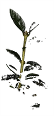
The first one (Figure 1(a)) contains a plant stalk with leaves. We try to differentiate between stalk and leaves. This data set mainly serves as baseline, as the shapes of stalk and leaves are different and thus, can be expected to be easy to distinguish. The scan contains a total of about 24 k points.

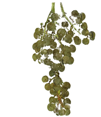
The second scan (Figure 1(b)) is a 360˚ scan of a grape bunch and consists of about 180 k points. We classify the points into parts of a berry or the stem skeleton that is visible in between. This distinction is important to be able to estimate the yield of grapes [2] [16] .

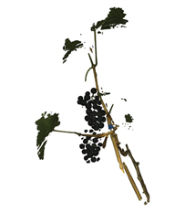
The third scan (Figure 1(c)) shows a grape branch, including stalks, leaves and a grape bunch, held by a supporting stick (about 100 k points total). We aim at a classification of the points in parts of the berry and the background, consisting of leaves, stalks and supporting stick. This is an extension of the grape scan.

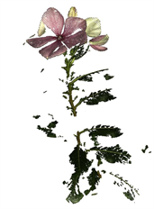
Finally, the last scan (Figure 1(d)) shows a flower represented by a number of about 47 k points. We aim at a classification of the points into parts of the petals

and the background, including leaves and stalk of the flower. This is the most challenging data set, as the chosen descriptors rely on the shape to differentiate the objects, but petals and leaves are rather similar. The only difference is a small curvature in the petals, while the leaves are more smooth. In many cases, the number of blossoms in a field already can be used as an early estimate of the yield. Therefore, differentiating between them and the background would be an important step.

We will refer to the scans as “Leaves”, “Grape”, “Branch” and “Flower” sets in the rest of the paper. All data sets were generated with the Artec Spider 3D scanner with a resolution of 0.1 mm and an accuracy of up to 0.05 mm [18] . The resolution was standardized using a voxelgrid filter with a voxel edge length of 0.5 mm. Especially leaves and flower data set, but the others as well, contain holes and occluded parts are missing, as has to be expected when scanning under natural conditions.

3.2. Classification

The performance of the descriptors is compared based on one supervised and one unsupervised approach.

For the supervised classification a Support-Vector-Machine (SVM) from the freely available svm-light library [19] with linear kernel, standard parameters and an inverse 10-fold cross validation was used. The training was done on one part of the data and validation of the model on the remaining nine parts. A gold standard was created manually for the leaves, branch and flower data set. This is very hard to do for grapes, as the stem structure is very fine and positioned between the berries. Therefore, we used a reconstruction approach based on sphere-RANSAC as presented in [2] with manual removal of erroneous berries for the grape data set.

The unsupervised classification is based on a k-means++ approach [20] using either the Euclidean or the χ²-distance between histograms. As the RoPS descriptor does not represent a histogram and, thus, can contain negative values, a normalization to $\left[\mathrm{0,1}\right]$ is carried out whenever the χ²-distance is applied.

We vary the number of cluster centres k as former examination showed that in some cases, even when only two types of objects are present in the data (like in our case in the grape and leaves data sets) using more cluster centres can be beneficial, as it allows for a finer clustering [13] . For the branch and flower data set, there is the additional reasoning that three types of objects exist in the data (stalks, leaves and berries for the branch data set and stalks, leaves and petals in the flower data set). While those objects are to be separated into only two classes (berries/petals and background), clustering into multiple classes and then manually assigning the clusters to the two classes promises to be more robust.

4. Results and Discussion

We optimize the radius parameters for normals (r_n) and support region (r) separately for each data set using a grid search on the SVM approach. The resulting best parameter combinations can be seen in Table 1.

In most cases, the tendency is the same for all parameters on the same data set. On branch, grape and leaves combinations of small r_n and great r lead to the best results. The flower data set is a special case, as the petals only differ from the leaves on a small scale (petals are slightly curved while leaves are rather smooth). Therefore, some descriptors tend to deliver better results if r is chosen relatively small. Only FPFH and SHOT remain stable with small r_n and great r over all data sets.

Former studies showed that as long as the bin sizes are set to sufficiently great values and a fitting distance measure is chosen, the bin sizes do not significantly influence the result [4] . Therefore, we used fixed values of 33 bins for the FPFHs, 125 bins for the PFHs, 352 for the SHOT descriptor, 135 for the RoPS and 153 for the Spin Images.

To judge the quality of the classification, the accuracy is computed on each data set, in the case of the SVM averaged over the 10 validation sets.

4.1. Supervised Classification

The accuracy achieved with a supervised classification is presented in Table 2.

On all data sets, the descriptors achieved results of more than 85% and taking out the challenging flower data set even more than 90%. Still, differences are visible.

The best results are achieved using the FPFHs. Even on the flower data set they yield more than 94% accuracy and up to over 99% on the branch data set.

The other descriptors perform comparably, with the RoPS descriptor and the Spin Images leading to the worst results, but still close to the others.

4.2. Unsupervised Classification

The accuracy achieved using a k-means clustering approach with either Euclidean or χ²-distance is depicted in Figure 2 for the leaves and grape data set and Figure 3 for the branch and the flower data set for varying numbers of cluster centres. Again, the FPFH is at the top on all data sets, mostly delivering the best results of all descriptors. Additionally, it is very robust, showing only slight changes after reaching a sufficient number of cluster centres. It is also interesting that even when using the Euclidean distance that is usually not a good choice for histograms, the same quality of results can be achieved. The reason for this is that the FPFHs require only a small number of bins (33), making the problems with noise usually occurring with the Euclidean distance less prominent.

The PFHs come close to the FPFHs in most cases, delivering better results on the flower data set, but worse on the branch data set.

Both RoPS and SHOT descriptor and Spin Images as well show bad results when using few cluster centres, only for more than four to six they stabilize. But even then, they do not achieve the same quality as PFHs and FPFHs. An exception is the branch data set, where the Spin Images perform almost as good as the FPFHs, but requiring more cluster centres.

All descriptors beside FPFHs and RoPS show a less robust behaviour when using the Euclidean distance compared to the χ²-distance. This suggests that for histogram descriptors with a greater number of bins (between 125 and 352) it is important to use a distance metric specific for histograms.

On the leaves and grape data set, all descriptors achieve good results of more than 85%. The branch data set is more challenging, but FPFHs and Spin Images both achieve more than 90%. On the flower data set, SHOT and RoPS descriptor and Spin Images as well fall below 80%. Only PFHs and FPFHs are able to get close to 90%.

4.3. Discussion

Both leaves and grape data set emerge to be rather simple classification problems, containing rather differently shaped plant organs. The branch data set provides a combination of the classes in the other data sets, being more challenging as more types of objects are included. The most problematic case is the flower data set.

The choice of the radius parameters proves to be dependent on the application. While the normal radius r_n can usually simply be set to a value equal or greater than the resolution, the support radius r has to be adjusted to the special requirements. If the plant organs that are to be distinguished vary only on a small scale, like on the flower data set, this has to be reflected by a smaller choice of r.

As expected, choosing an SVM as more sophisticated classification method makes the choice of the descriptor almost irrelevant, as all of them achieve very good results. But for an SVM, a gold standard has to be prepared and depending on the use case, this can be hard (e.g. the labelling of the stem skeleton inside a grape bunch is almost impossible to do manually). Fortunately, even in the case of unsupervised classification FPFHs yield very good results.

The evaluation on the representative sets shows a clear ranking for the SVM-based classification: FPFHs perform best, while the other descriptors all yield results similar to each other. In the case of the k-means clustering, we have on average the following ranking: FPFHs > PFHs > Spin Images > RoPS, SHOT. There are slight deviations, e.g., the Spin Images show the worst results of all descriptors on the Leaves data set, but reach almost the same quality of results as FPFHs on the Branch data set. The same effect can be seen in the SVM results. This suggests that the resolution chosen for the Spin Images in this paper is better suited to distinguish between round and flat or cylindrical shapes than between flat and cylindrical shapes only.

All in all and despite the exemplary character of the evaluation the results clearly suggest using FPFHs as descriptor of choice when compared with SHOT, RoPS and Spin Images.

In applications like scan registration, both RoPS and SHOT descriptor were found to outperform PFHs and FPFHs [8] [9] . In contrast to that, we strive to classify the whole set of points and assign them to the corresponding plant organ. This means that the descriptor has to be able to generalize over different sizes of plant organs. Additionally, scans can not be expected to be perfect, as they have to be taken in the field and for a high number of plants. Parts of the plant can be occluded by other parts and holes in the data are possible. The descriptor has to be robust against these issues. The good performance of the FPFHs and PFHs in our application together with the worse performance of RoPS and SHOT descriptors therefore hints that FPFHs and PFHs seem to have the generality that makes them less suitable for applications where different points on a similar shaped surface have to be distinguished, but optimal for point classification in the context of precision farming.

5. Conclusion and Future Work

In this work, the performance of different descriptors and classification methods in the context of precision farming is shown, represented by four typical settings, including the distinction between leaves, stalks and berries. When using a supervised classification with an SVM, the FPFHs lead to the best result in a tight ranking with the other descriptors. The results achieved with unsupervised k-means clustering show an even more distinct tendency: while the performances of the other descriptors drop, FPFHs still yield results comparable to supervised classification.

So far, we presented experimental results on one representative scan for each type of scan data. To validate our conclusions, the same experiments should be done on a much higher number of data sets.

Furthermore, a reconstruction of plant organs with geometric primitives could be applied to the classified data to derive phenotypes e.g. for yield estimation directly from 3D input data.

Acknowledgement

This work was done within the project “Automated Evaluation and Comparison of Grapevine Genotypes by means of Grape Cluster Architecture” which is supported by the Deutsche Forschungsgemeinschaft (funding code: STE 806/2-1). We thank the DFG for supporting our work.

Cite this paper

Mack, J., Trakowski, A., Rist, F., Herzog, K., Töpfer, R. and Steinhage, V. (2017) Experimental Evaluation of the Performance of Local Shape Descriptors for the Classification of 3D Data in Precision Farming. Journal of Computer and Communications, 5, 1-12. https://doi.org/10.4236/jcc.2017.512001

References

- 1. Furbank, R.T. and Tester, M. (2011) Phenomics Technologies to Relieve the Phenotyping Bottleneck. Trends in Plant Science, 16, 635-644.
- 2. Mack, J., Lenz, C., Teutrine, J. and Steinhage, V. (2017) High-Precision 3D Detection and Reconstruction of Grapes from Laser Range Data for Efficient Phenotyping Based on Supervised Learning. Computers and Electronics in Agriculture, 135, 300-311.
- 3. Roscher, R., Herzog, K., Kunkel, A., Kicherer, A., Topfer, R. and Forstner, W. (2014) Automated Image Analysis Framework for High-Throughput Determination of Grapevine Berry Sizes Using Conditional Random Fields. Computers and Electronics in Agriculture, 100, 148-158.
- 4. Behley, J., Steinhage, V. and Cremers, A.B. (2012) Performance of Histogram Descriptors for the Classification of 3D Laser Range Data in Urban Environments. IEEE International Conference on Robotics and Automation (ICRA), Saint Paul, MN, 14-18 May 2012, 4391-4398.
- 5. Guo, Y.L., Sohel, F., Bennamoun, M., Lu, M. and Wan, J.W. (2013) Rotational Projection Statistics for 3d Local Surface Description and Object Recognition. International Journal of Computer Vision, 105, 63-86.
- 6. Alexandre, L.A. (2012) 3D Descriptors for Object and Category Recognition: A Comparative Evaluation. IEEE International Conference on Intelligent Robotic Systems (IROS), Workshop on Color-Depth Camera Fusion in Robotics, October 2012, 1-6.
- 7. Rusu, R.B., Marton, Z.C., Blodow, N. and Beetz, M. (2008) Learning Informative Point Classes for the Acquisition of Object Model Maps. International Conference on Control, Automation, Robotics and Vision (ICARCV), December 2008, 643-650.
- 8. Yang, J.Q., Cao, Z.G. and Zhang, Q. (2016) A Fast and Robust Local Descriptor for 3D Point Cloud Registration. Information Sciences, 346-347, 163-179.
- 9. Yang, J.Q., Zhang, Q., Xian, K., Xiao, Y. and Cao, Z.G. (2016) Rotational Contour Signatures for Robust Local Surface Description. IEEE International Conference on Image Processing, September 2016, 3598-3602. https://doi.org/10.1109/ICIP.2016.7533030
- 10. Tombari, F., Salti, S. and Di Stefano, L. (2010) Unique Signatures of Histograms for Local Surface Description. European Conference on Computer Vision, September 2010, 356-369.
- 11. Rusu, R.B., Blodow, N. and Beetz, M. (2009) Fast Point Feature Histograms (FPFH) for 3D Registration. IEEE International Conference on Robotics and Automation, 3212-3217. https://doi.org/10.1109/ROBOT.2009.5152473
- 12. Paulus, S., Dupuis, J., Mahlein, A.-K. and Kuhlmann, H. (2013) Surface Feature Based Classification of Plant Organs from 3D Laser Scanned Point Clouds for Plant Phenotyping. BMC Bioinformatics, 14, 238. https://doi.org/10.1186/1471-2105-14-238
- 13. Wahabzada, M., Paulus, S., Kersting, K. and Mahlein, A.K. (2015) Automated Interpretation of 3D Laser Scanned Point Clouds for Plant Organ Segmentation. BMC Bioinformatics, 16, 248-258.
- 14. Johnson, A.E. and Hebert, M. (1999) Using Spin Images for Efficient Object Recognition in Cluttered 3D Scenes. IEEE Transactions on Pattern Analysis and Machine Intelligence, 21, 433-449.
- 15. Rusu, R.B. and Cousins, S. (2011) 3D Is Here: Point Cloud Library (PCL). IEEE International Conference on Robotics and Automation, May 2011, 1-4. https://doi.org/10.1109/ICRA.2011.5980567
- 16. Rose, J.C., Kicherer, A., Wieland, M., Klingbeil, L., Topfer, R. and Kuhlmann, H. (2016) Towards Automated Large-Scale 3D Phenotyping of Vineyards under Field Conditions. Sensors, 16, 2136.
- 17. Marton, Z.C., Rusu, R.B. and Beetz, M. (2009) On Fast Surface Reconstruction Methods for Large and Noisy Datasets. Proceedings of the IEEE International Conference on Robotics and Automation, Kobe, 12-17 May 2009.
- 18. Artec 3D (2017). https://www.artec3d.com/3d-scanner/artec-spider
- 19. Joachims, T. (1999) Making Large-Scale SVM Learning Practical. In: Scholkopf, B., Burges, C. and Smola, A., Eds., Advances in Kernel Methods Support Vector Learning, Chapter 11, MIT Press, Cambridge, 169-184.
- 20. Arthur, D. and Vassilvitskii, S. (2007) K-Means++: The Advantages of Careful Seeding. In: Proceedings of the Eighteenth Annual ACM-SIAM Symposium on Discrete Algorithms, Society for Industrial and Applied Mathematics, Philadelphia, 1027-1035.