Journal of Computer and Communications
Vol.2 No.5(2014), Article ID:43586,28 pages DOI:10.4236/jcc.2014.25001
Knowledge Discovery in Data: A Case Study
Ahmed Hammad1, Simaan AbouRizk2
1HMD Project & Knowledge Management Services, Edmonton, Canada
2Department of Civil and Environmental Engineering, Hole School of Construction Engineering and Management, University of Alberta, 3-014 Markin/CNRL Natural Resources Engineering Facility, Edmonton, Alberta, Canada
Email: ahmed.hammad@worleyparsons.com, abourizk@ualberta.ca
Copyright © 2014 by authors and Scientific Research Publishing Inc.
This work is licensed under the Creative Commons Attribution International License (CC BY).
http://creativecommons.org/licenses/by/4.0/


Received 13 December 2013; revised 10 January 2014; accepted 18 January 2014
ABSTRACT
It is common in industrial construction projects for data to be collected and discarded without being analyzed to extract useful knowledge. A proposed integrated methodology based on a five-step Knowledge Discovery in Data (KDD) model was developed to address this issue. The framework transfers existing multidimensional historical data from completed projects into useful knowledge for future projects. The model starts by understanding the problem domain, industrial construction projects. The second step is analyzing the problem data and its multiple dimensions. The target dataset is the labour resources data generated while managing industrial construction projects. The next step is developing the data collection model and prototype data warehouse. The data warehouse stores collected data in a ready-for-mining format and produces dynamic On Line Analytical Processing (OLAP) reports and graphs. Data was collected from a large western-Canadian structural steel fabricator to prove the applicability of the developed methodology. The proposed framework was applied to three different case studies to validate the applicability of the developed framework to real projects data.
Keywords:Construction Management; Project Management; Knowledge Management; Data Warehousing; Data Mining; Knowledge Discovery in Data (KDD); Industrial Construction; Labour Resources

1. Introduction
Many industrial construction projects face delays and budget overruns, often caused by improper management of labour resources [1] . The nature of industrial construction projects makes them more complicated: a large number of stakeholders with conflicting interests, sophisticated management tools, stricter safety and environmental concerns.
In the changing environment, each involved contractor simultaneously manages multiple projects using one pool of resources. During this process, a large amount of data is generated, collected, and stored in different formats, but it is not analyzed to extract useful knowledge. The improvement of labour management practices could have a significant impact on reducing schedule delays and budget overruns. One solution to this problem is analysis of historical labour resources data from completed projects to extract useful knowledge that can be transferred and used to improve resource management practices.
Data warehouses are one method often used to extract useful knowledge. They are dedicated, read-only, and nonvolatile databases that centrally store validated, multidimensional, historical data from Operation Support Systems (OSS) to be used by Decision Support Systems (DSS) [2] . Data warehouses are typically structured either on the star schema, consisting of a fact table that contains the data and dimension tables that contain the attributes of this data, for simple datasets, and on the snowflake schema, used either when multiple fact tables are needed or when dimension tables are hierarchical in nature [3] , for complicated datasets. A data warehouse typically consists of three main components: the data acquisition systems (backend), the central database, and the knowledge extraction tools (frontend) [4] . On Line Analytical Processing (OLAP) techniques (roll-up and drill-down, slice and dice, and data pivoting) are typically used in the frontend of a data warehouse to present end-users with a dynamic tool to view and analyze stored data.
Data mining is “the analysis of observational datasets to find unsuspected relationships and to summarize the data in novel ways that are both understandable and useful to the data owners” [5] . Considering data mining, the knowledge discovered must be previously unknown, non-trivial, and useful to the data owners [6] . Data mining techniques rely on either supervised or unsupervised learning and are grouped into four categories [7] . Clustering methods minimize the distance between data points falling within a cluster, and maximize the distance between these clustered data points and other clusters [8] . Finding Association Rules highlights hidden patterns in large datasets. Classification techniques, including Decision Trees, Rule-Based Algorithms, Artificial Neural Networks (ANN), k-Nearest Neighbours (k-NN or lazy learning), Support Vector Machine (SVM), and many others, build a model using a training dataset to define data classes, evaluate the model, and then use the developed model to classify each new data point into the appropriate class [7] . Outliers’ detection techniques focus on data points that are significantly different from the rest.
Data warehousing and mining techniques have been applied to solve problems in the construction industry over the last decade. However, none of the previous research applied these techniques to address management of multiple projects simultaneously using one common pool of labour resources; the problem is typically solved using other techniques (Heuristic rules, Numerical Optimization and Genetic Algorithms). Most previous research focused on leveling or allocating resources in a single project environment. Soibelman and Kim [9] analyzed schedule delays with a five-step KDD approach. Chau et al. [10] developed the Construction Management Decision Support System (CMDSS) by combining data warehousing, Decision Support Systems (DSS) and OLAP. Rujirayanyong and Shi [11] developed a Project-oriented Data Warehouse (PDW) for contractors, but it was limited to querying the warehouse without using data mining. Moon et al. [12] used a four-dimension cost data cube in their application of Cost Data Management System (CDMS), built using MS SQL Server-OLAP Analysis Services, to obtain more reliable estimates of construction costs. Fan et al. [13] used the Auto Regression Tree (ATR) data mining technique to predict the residual value of construction equipment.
In this research, the Cios et al. [7] hybrid model was modified and adapted to develop an integrated methodology for extracting useful knowledge from collected labour resources data in a multiple-project environment utilizing the concepts of KDD, data warehousing, and data mining. When the techniques are integrated, they combine quantitative and qualitative research approaches and facilitate working with large amounts of data impacted by a large number of unknown variables, which was integral to this research. Further information on the developed framework can be found in Hammad et al. [14] . The proposed integrated methodology based on a five-step Knowledge Discovery in Data (KDD) model is shown in figure 1.
In this paper, the proposed modified hybrid KDD model is applied to three different case studies to test its ability to extract useful knowledge from datasets. Section 2 discusses discovering knowledge in the first dataset; Section 3 covers the second dataset and Section 4 the third dataset. The paper outlines the process of applying the model to extract data, the related procedures, and outlines the useful data collected.
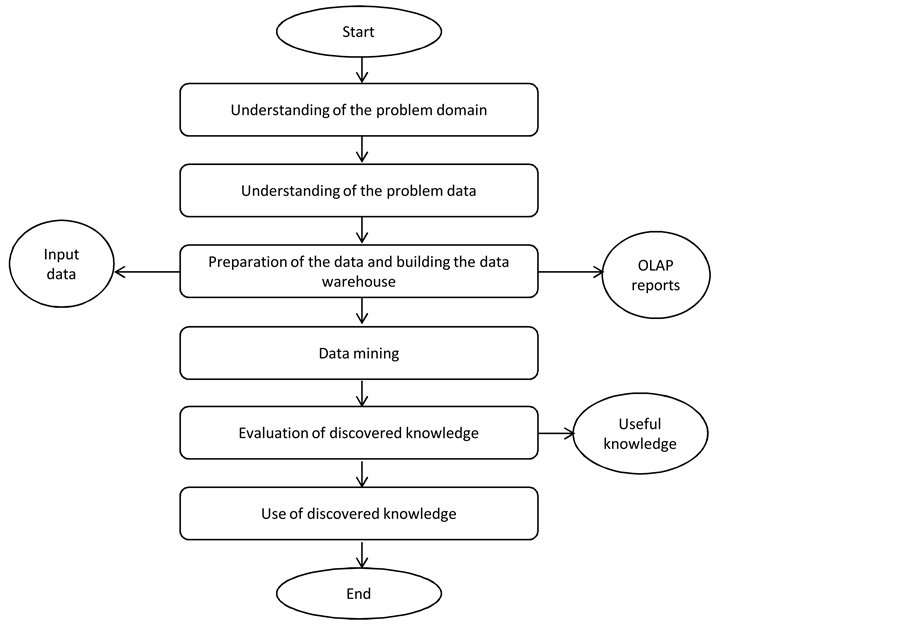
Figure 1. Modified hybrid KDD model.
2. Discovering Knowledge in the First Dataset
2.1. Data Cleaning and Preprocessing
This paper shows how to implement data mining techniques to extract useful knowledge from three datasets that were obtained from real projects. The purpose of this case study is to validate that data mining can be used to improve and increase the efficiency of labour estimating practices in contracting companies. Most of these companies rely on cost estimating units (norms) that are not based on historical data and are not updated to reflect changes in the industry. Applying the proposed approach that relies on data mining is expected to provide companies with knowledge-based probabilistic dynamic estimating units that always reflect the latest changes.
The first dataset contains data regarding the scope of a set of engineering work packages. This scope is represented as determinate amounts of key quantities per work package. The key quantity for engineering packages is the number of engineering deliverables. The dataset was obtained from the estimating system of the participating contractor. This estimating system is based on an old version of MS Access. The dataset contains the original and current baseline hours for five of the involved resources in this group of work packages. The current baseline values reflect the project scope after implementing all approved changes. The selected dataset to be analyzed in this case study contained data for more than one hundred projects, four project phases and five different resources.
The contractor did not track actual hours spent per work package; however, the same analysis can be easily applied if the data exists. The analysis was used to check the consistency of the estimating practices in this contracting company. The data was directly exported from the estimating system to MS Excel, where the cleaning and preprocessing took place prior to exporting the data to the data warehouse. Figure 2 shows an example of the raw data. Data was found to be missing, and also, metadata (data about the data) was missing. The data lacked the values for two important control attributes: the internal program and the project phase, and had to be assigned manually.
This manual procedure required going back to the archived project documents to find the appropriate values
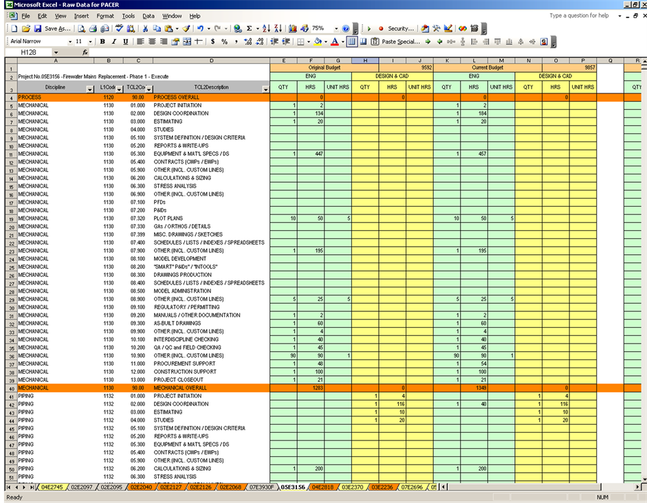
Figure 2. The raw data for the first data set.
to be assigned to each data point. Completing and verifying the dataset required ample time and effort. Furthermore, while working with the archived documents, some documents were not clear enough and assumptions had to be made to compensate for the missing data. Many of the staff members who were involved in these projects could not be located, and if they could be contacted, they could not provide meaningful input on the data as time has passed. All the effort and time spent searching, sorting, and cleaning in the archive would have been easily avoided if the data and its metadata were collected in the proposed integrated format.
Figure 3 shows the data from Figure 2 after it was cleaned, pre-processed and ready for storage in the data warehouse. The objective of this analysis was to test if the resource unit cost per production package type could be extracted for future estimating of resource requirements in upcoming projects. For this analysis, fifteen standard production packages, three engineering phases and five engineering resources were selected. The data was modified by random numbers for confidentiality issues. This modified data was used in the analysis. Hence, all numbers shown here are used only for illustration.
Three control attributes were selected for this analysis. These control attributes were represented in this analysis with the independent variables: Package(1:15), Phase(1:3) and Resource(1:5). These are nominal variables with values assigned to them as discrete integers. These discrete integers were equal to the ID’s used in the data warehouse for direct referencing. To test the significance of adding more attributes to the analysis, the internal program control attribute was selected. This attribute is represented in the analysis with the independent variable Program(1:3).
In this study, the term “class” refers to a unique combination of values of the three variables: package, phase and resource. For example, class 1 contains all the data points that have the value Pk(1) for the variable package, Ph(1) for the variable phase and R(1) for the variable resource. A class 2 contains all the data points that have the
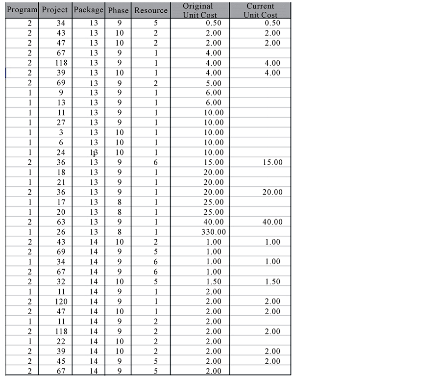
Figure 3. The dataset after cleaning and pre-processing.
value Pk(1) for the variable package, Ph(1) for the variable phase and R(2) for the variable resource, etc. The number of classes resulting from all the possible combinations is calculated using the formula:
 (1)
(1)
It is important to note that the dataset may not include data points for all the classes. Certain classes of the three main attributes do not exist in reality. For example, some packages are not needed in every phase, or some packages do not utilize all the five resources under investigation.
The key quantity for all the packages is the number of engineering deliverables. This analysis is implemented to the hourly portion of the collected data, since estimating of labour resource requirements relies on hourly units and not on cost. The dataset was normalized to eliminate the differences in project sizes by calculating three dependent variables: “Original Hourly Unit Cost,” “Current Hourly Unit Cost,” and “Actual Hourly Unit Cost.” These variables are calculated using the following formulas:
 (2)
(2)
 (3)
(3)
 (4)
(4)
Because of the multidimensionality of this dataset, four new variables were formulated to represent the possible combinations of the three main attributes. These new variables were Package/Phase, Package/Resource, Phase/Resource and Package/Phase/Resource. These variables were assigned unique values by combining ID's from the three main attributes.
After defining all the necessary variables, the dataset was then exported to the first analysis tool, SPSS-16 for Windows. SPSS was selected because of its ability to perform a wide range of statistical analysis tests, its ability to easily import and export data from databases and its user friendliness. It can be easily obtained by any contractor or industrial owner who needs to perform statistical analysis of the collected data in the data warehouse.
The objective of this analysis was to develop an estimating methodology to be implemented using unit costs and key quantities. First, the dataset was divided into clusters using stratification. Significant differences of means are used to establish these clusters. Within each cluster, unit cost and the characteristics of the most fitting distribution are obtained. Therefore, instead of relying solely on their intuitions, the estimators are presented with mined values for the unit costs that can be multiplied by the known determinate key quantities in order for these estimators to predict the resource requirements more accurately.
2.2. The Initial Investigation
Data mining models suggest starting any exercise with visual presentation of the available dataset. First, the frequency of data points within each independent variable is plotted. Figure 4 graphically shows that phase Ph-03 had more data points than the other two phases. Figure 5 shows that not every package utilized the five resources and that some packages only utilize a single resource.
Second, the data descriptive ‘case summaries’ test is performed to collect statistics on each class or data subset. Since the data is multidimensional, subsets can be generated using one attribute, a combination of any two attributes, or all three attributes combined. The following statistics are obtained: mean, standard deviation, number of data points, minimum value, maximum value and data range. Figure 6 shows an excerpt of the test results.
Subsequently, statistical dispersion is measured using boxplots that are obtained for each of the data subsets. Boxplots show the Inter Quartile Range - IQR (the 25th percentile, the median, 75th percentile) minimum, maximum and extreme values. SPSS points to the raw number that contains data points that are out of the normal range.
The descriptive statistics as well as the boxplots showed very wide ranges and variance (Figures 7 and 8). They also showed that the dataset contains extreme outliers. As a result of this situation, it was necessary to implement an outlier detection procedure.
2.3. The Outliers Detection Procedure
Given that the boxplot results showed outliers in the dataset, detecting them was necessary. In this research, the technique implemented was based on Chebyshev Theorem [15]. This theorem can be used for single dimension (univariate) outliers analysis. Assuming the dataset follows a normal distribution, the mean and standard deviation of the distribution can be defined by calculating the mean (µ) and standard deviation (σ) of the dataset. Chebyshev stated that since most data points fall between (µ + 3σ) and (µ − 3σ), those that fall outside of this range can be considered outliers.
A four layer outlier analysis tool was developed based on the three-dimensional dataset.
• First layer = all data Second layer = each attribute
• Third layer = three possible combinations of paired attributes represented as three new category variables (package * phase provides 45 combinations, package * resource provides 75 combinations and phase * resource provides 15 combinations).
• Fourth layer = all attributes combined (provides 225 combinations) represented as new category variable.
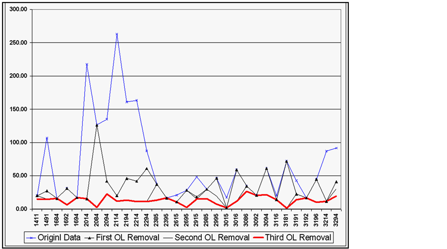
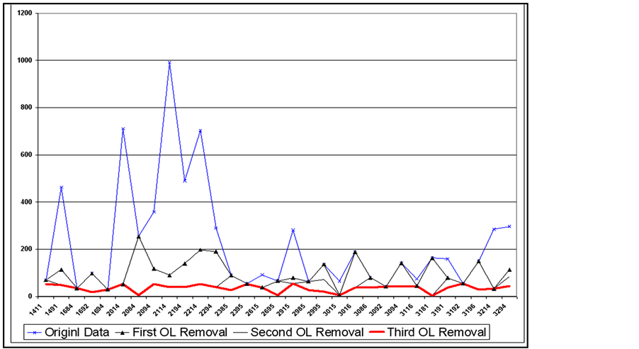
A total of eight possible cases of outliers were calculated using the obtained means and standard deviations obtained from SPSS. Each data point was tested against the eight cases and was assigned a value of 1 if found to be an outlier in any case. A total outlier score is calculated by adding the number of cases where a data point was an outlier. An example of the output is shown in Figure 9. It is up to the user to go back and verify the outliers or eliminate them and perform the analysis. The procedure was repeated three times until the obtained standard deviations and ranges were found to be acceptable as shown in Figures 10 and 11.
Cases with less than three data points were eliminated from the analysis. The mean and standard deviation of
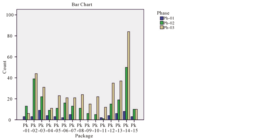
Figure 4. Frequency of data points within the three phases.
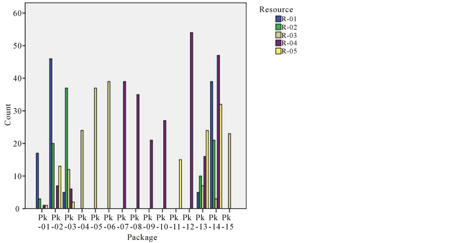
Figure 5. Frequency of data points within the five resources.
every class was calculated and summarized graphically on a tree, as shown in Figure 12. The user can now use the summary tree to find out the unit cost multiplier distributions to be used for estimating new projects in the future. For each layer, a new variable Select (K) is assigned to each data point, where k = layer number.
Instead of using the mean and standard deviation of the normal distribution, the user can also use fitting-distribution software such as @Risk to find the most fitting distribution for the data in a class. Figure 13 shows an example of finding the most fitting distribution for one of the classes.
2.4. Clustering of Unit Cost using Statistical Methods
Building the unit cost tree shows a large number of classes, which can drastically increase if more variables are
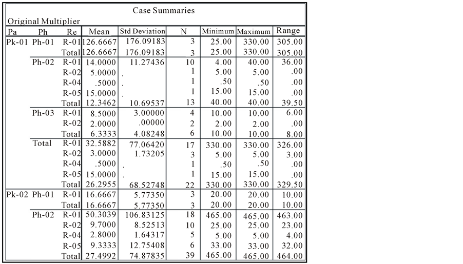
Figure 6. The descriptive data test.

added to the dataset. To simplify the estimating procedure, classes that are not significantly different from each other are combined together in summary groups (clusters) with one distribution representing each cluster. The ANOVA test was implemented to the dataset to check the significance of mean differences within the seven data attributes and the results are shown in Figure 14.
The results for the Post Hoc tests for the three main attributes with α = 0.05 are shown in Figure 15.
If the user decides to use only one attribute for dividing the dataset, test results in Figure 15 show that pack-

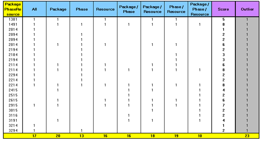
Figure 9. The output from the outlier detection tool.
ages can be grouped into four classes, phases can be grouped into two classes and resources can be grouped into two classes.
If the user decides to use the combination of the three main attributes (Package * Phase * Resource), Figure 16 shows the Post Hoc test results for this combination. The test results are used to group the classes into eight clusters and a new variable Cluster(1:8) is assigned to each data point. The case summary and Boxplot tests were repeated and the results are shown in Figure 17 and Figure 18.
Figure 19 shows the dataset in SPSS after assigning all the analysis variables. That dataset can be used for a lot more tests if more data and attributes are available. The simplicity of the analysis and the techniques used in it opens the door for the end user to continue searching for more patterns and hidden knowledge in the collected
data.
This case study presents the value of obtaining the unit costs from historical data using data mining. It shows that extracting useful knowledge from data can be maximized if all data elements are collected properly. Two major problems pertinent to the dataset were found. First, discrepancies were found among the different estimators’ entries. Estimators are supposed to enter both the estimated quantity of a deliverable and the estimated amount of unit hours per quantity item. The system would then calculate the total estimated hours for a package. However, this was not the case for all data points. Some estimators did not provide estimated quantity; they only put the number T in the quantity field. This practice, hence, led to erroneous hourly unit estimation.
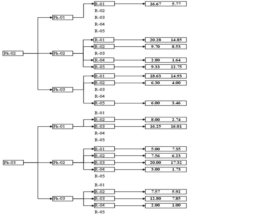
Figure 12. The output summary tree.
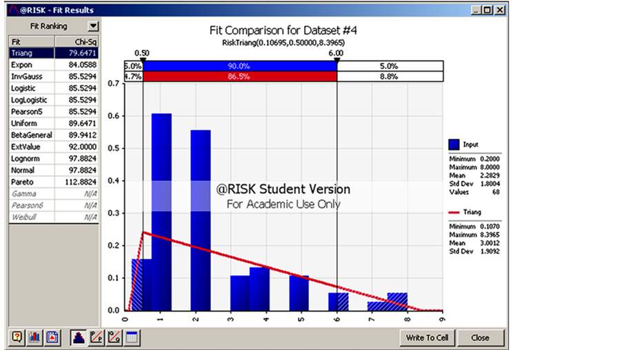
Figure 13. Fitting distribution to a class of data.
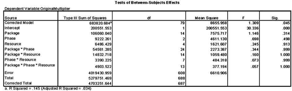
Figure 14. Univariate ANOVA test results for the three main attributes.
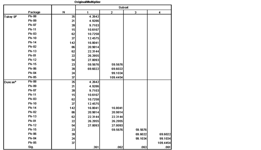
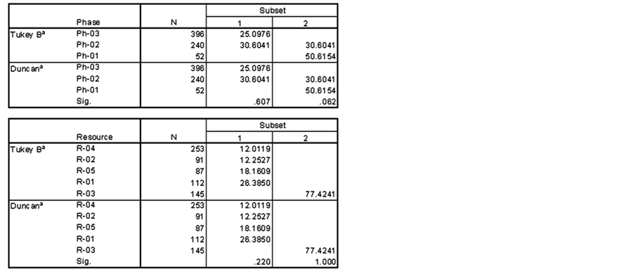
Figure 15. Post hoc test results for the three main attributes.
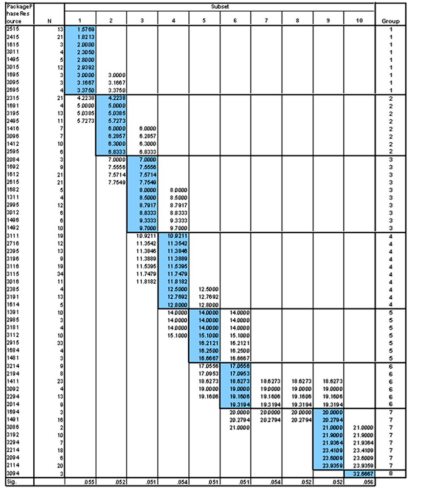
Figure 16. Duncan test results.
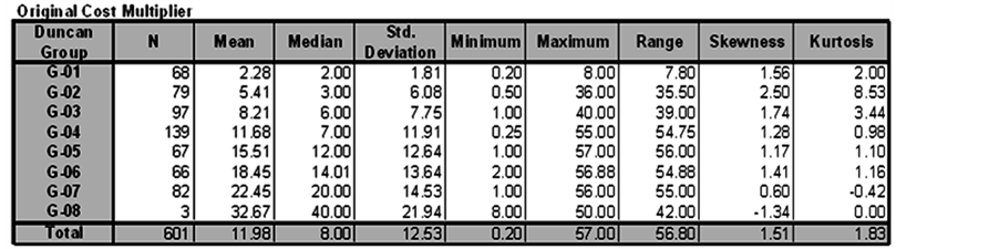
Figure 17. Statistical analysis for the eight data clusters.
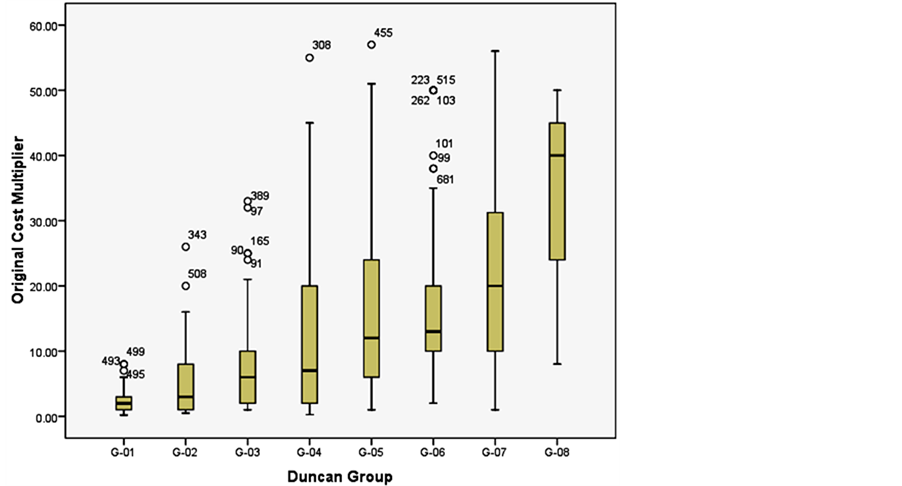
Figure 18. Box Plots for the eight data clusters.
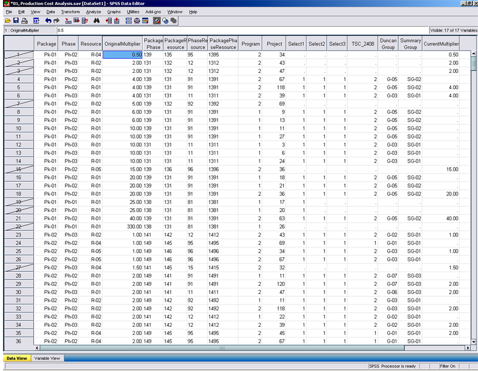
Figure 19. The final dataset with the select and cluster variables.
Another source of discrepancy was found in the estimating of hours required to complete work packages. Some estimators included all the support activities, such as meetings, site visits and quality inspections, in their production package estimates. Others estimated the requirement for the support activities independently from the production packages. Again, this led to erroneous hourly unit estimates of production packages.
In addition to the discrepancies found in the estimating entries, discrepancies were found in recording actual entries. The actual hours spent were collected at the project level, as opposed to the planning hours that were estimated at the work package level. Given the levels where the data was collected, there was no possibility to compare or analyze the variance between the estimated and the actual hours spent. Similar to the estimated dataset, the actual dataset should have been collected at the work package level.
These discrepancies caused inconsistencies in the data. When the dataset was analyzed, large amount of outliers caused significant disparity in the results. These outliers were highlighted using the outlier detection tool developed in this research and were presented to the data owner for corrective action. Two recommendations were made to the company about these issues, and were approved to be implemented: first, to issue estimating guidelines to ensure consistency among different estimators; second, to modify the timekeeping system in a way to collect actual hours spent at the work package level.
3. Discovering Knowledge in the Second Dataset
3.1. Data Gathering, Cleaning and Preprocessing
The purpose of this case study is to validate the concept that mining historical data enables contractors to better estimate the duration of their work packages. Current practices rely mostly on estimating the duration by dividing the total work hours by the daily number of hours or the scheduler experience. Both practices struggle to provide reliable estimates of package durations that utilize prior experience and current project conditions.
The second dataset used in this research contains actual duration and working hours for a large group of fabrication work packages. This dataset included 13,498 data points and was obtained from the second partner company. This company is a large EPC firm that specializes in fabricating structural steel for industrial construction projects. The data was obtained from the scheduling information system of this company, which is a SQL-Server database that was originally designed by the author and developed by the NSERC Industrial Research Chair in Construction Engineering and Management. The data was automatically extracted out of the SQL-Server data tables to MS Excel for cleaning and preprocessing.
The researcher helped the contractor to develop a predefined set of progress activities for their fabrication packages. The start and finish date for each one of these progress activities were collected over a long period of time. The actual steel weight and working hours to complete each fabrication package were also stored in the information system. The steel weight represents the key quantity for each of these work packages. However, the production package (work package type) was not assigned to the obtained dataset.
The cleaning procedure started by selecting the data point that represents the completed work packages, which means start-date and end-date were marked actual. After that, the obvious data entry errors, such as negative values, were also eliminated.
The data for handrails and miscellaneous very small fabrication packages were eliminated as well, because they are handled by a separate facility, and are not in the scope of this data-mining exercise. After the cleaning procedure, a large dataset with 5590 data points was still available to analyze. The duration (D) (n) in work weeks was calculated using the formula:
 (5)
(5)
Figure 20 shows the data from Figure 21 after it was cleaned, pre-processed and was ready for storage in the data warehouse.
3.2. Clustering of the Cost and Duration Units
This second dataset contained more than five thousand work packages for two standard phases: shop drawings and fabrication. The actual quantities of deliverables, hours and weeks spent on each package was recorded. The fabrication and shop drawings hourly unit cost and weekly unit duration are calculated for every work package in the dataset. This data was collected over a long period of time. This data had not been analyzed or used before

Figure 20. Raw dataset for the second analysis.
for data mining or knowledge discovery.
The purpose of the analysis of this data was to use historical data to develop realistic, reliable and more accurate estimating units for both resource requirement and expected duration. These estimating units were then multiplied by the known quantities to estimate the total duration and resource requirement of a work package.
Since this data is based on actual values, the dataset has been used to validate the developed estimating methodology in this research. The dataset was divided into two parts. The first part, consisting of 85% of the data points, was selected randomly and used for calculating the estimating units. The second part, the remaining %15 of the data points, was used for testing purposes.
The software selected to perform the analysis is called Weka (Waikato Environment for Knowledge Analysis), which is a powerful and user friendly data mining and machine learning tool. Weka was developed at the University of Waikato in Hamilton, New Zealand [16] . The software was selected because of its powerful data mining capabilities. The software is also easy to obtain, and doesn’t require any special hardware; therefore, it would be accessible to any contractor seeking to perform data mining without incurring major cost. Minimizing the cost of implementing data mining in industrial construction makes it more appealing to decision makers and also maximizes the return on investment of the increased efficiency.
Weka is able to read data from different types of data files. The first 85% of the dataset was exported from the data warehouse to a Comma Separated Values (CSV) file. Then, it was transferred to Weka in order to perform the analysis. The data contained a unique ID for each data point, two control variables: program and project, the actual amount of key quantity, and total hours and weeks for two resources. One resource is utilized during the fabrication phase and the other one is utilized during the shop drawings phase. The unit cost was calculated by dividing total hours by the key quantity. The unit duration was calculated by dividing the total number of weeks by the key quantity. An excerpt of the CSV data file for the fabrication resource is shown in Figure 22.
Unlike the first dataset where several resources in multiple phases with different package type were analyzed
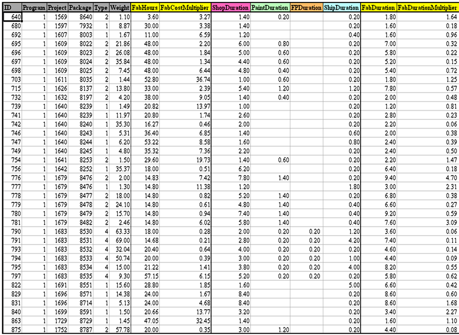

Figure 22. An excerpt of the CSV data file for the fabrication phase.
simultaneously, for this dataset, the analysis is done on one single resource per phase. Since there is no data collected regarding production package type, the data was analyzed with the assumption that it is all under one production package type. For this analysis, clustering, which is an unsupervised learning technique, was selected. Among the several clustering techniques available in Weka that were tested, the Expectation Maximization (EM) technique was found to be the most efficient one. The software developers highly recommend this technique for clustering large sets of data and it is the default technique to be used.
The EM clustering technique is applied to the dataset and the results are summarized in Figures 23-26. In order to ensure the stability of the clustering results, each clustering analysis was repeated three times, with each run taking about two and half hours of processing time on an Intel Pentium(R) personal computer. The results were as follows: nineteen clusters were obtained for the fabrication hourly unit cost (Figure 23), thirteen clusters for the fabrication weekly unit duration (Figure 24), five clusters for the shop drawings hourly unit cost (Figure 25) and six clusters for the shop drawings weekly unit duration (Figure 26). For each cluster, the number of data points, mean, standard deviation, and prior probability are obtained from Weka.
Initial results of the clustering exercise demonstrate trends that would benefit the contractor. Clusters with a large number of data points are expected to represent common cases of packages in the contracting company, while clusters with a small number of data points represent either rare types of work packages or outliers that have to be further investigated.
For instance, results in Figure 23 show that almost a quarter of the work packages fall in cluster 13, with a mean of 0.6 hours per unit. In the same table, packages in cluster 7 represent a case of outliers that should be investigated. When a contractor needs to investigate the clustering analysis results, they can easily find out which data point belongs to which cluster, since Weka assigns the results of the clustering to every data point in the dataset and automatically draws the frequency histograms as shown in Figures 27 and 28. Assigning clusters to every data point makes it easy for contractors to go back to their files and find out the reasons behind the variation in actual package cost and durations.
The Weka analysis supports the claim of this research model that data, which up to now was not used, can be transferred into useful knowledge that ultimately provides meaningful insights into the work of contractors. When data is collected, stored and pre-processed in a proper way, as proposed in this research, an endless wealth of knowledge can be harvested from this data. After assigning the clusters, a fitting distribution can be found for each cluster.
3.3. Case Study Results Validation
The second part of the data, the remaining 15% was used for validation, as mentioned earlier. The obtained unit costs and durations from the clustering analysis were used to estimate the resource requirement and duration of each work package in the validation dataset. Each package was assigned a duration unit cluster and a cost unit cluster (Figure 29). The means of these two clusters were used to estimate the total resource requirement and duration for each package.
Both the cost and duration variances, accompanied with error percentages, were calculated for each package as well.
The validation test showed that, when comparing the estimated values using the obtained unit based on historical data with the actual values that were recorded for these packages, more than 80% of the tested data points had an estimating error of below 25%. These results demonstrate a significant increase in the accuracy of estimating practices when relying on historical data that existed already in the contractor's management systems.
The work package types were not identified when the data was recorded. When the data mining analysis was conducted, data clusters were identified. Consequently, it was left to the estimator to decide which cluster to use for estimating future projects. The partner company did not record its planned data in a structured way as it did with the actual data. Thus, performance evaluation using EVM was not possible.
4. Discovering Knowledge in the Third Dataset
4.1. Data Gathering, Cleaning and Preprocessing
The purpose of this case study was to validate the concept that data mining can be used to provide reliable probabilistic resource utilization graphs (resource baseline histograms) that can be used for proper staffing of
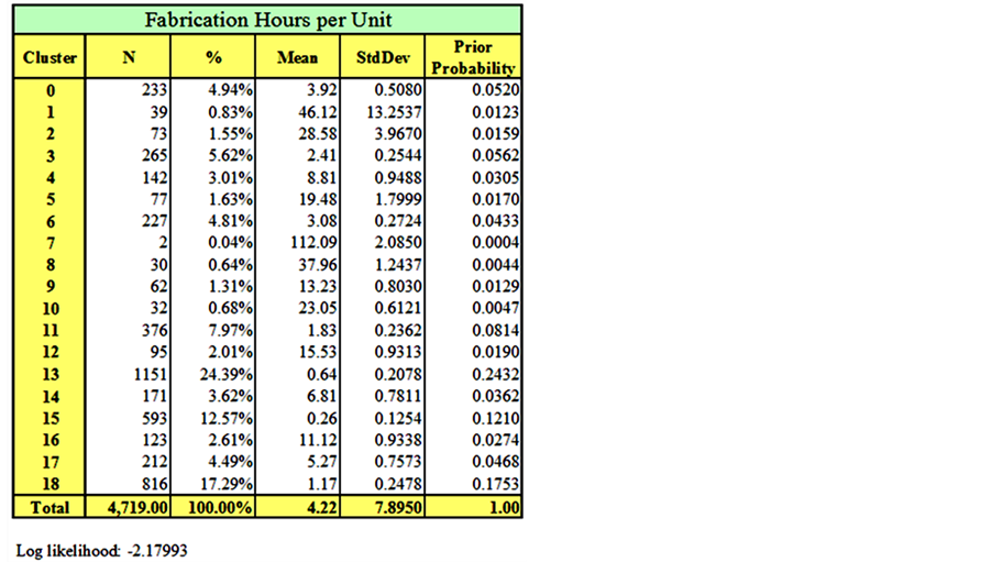
Figure 23. Clustering of fabrication hourly unit cost.
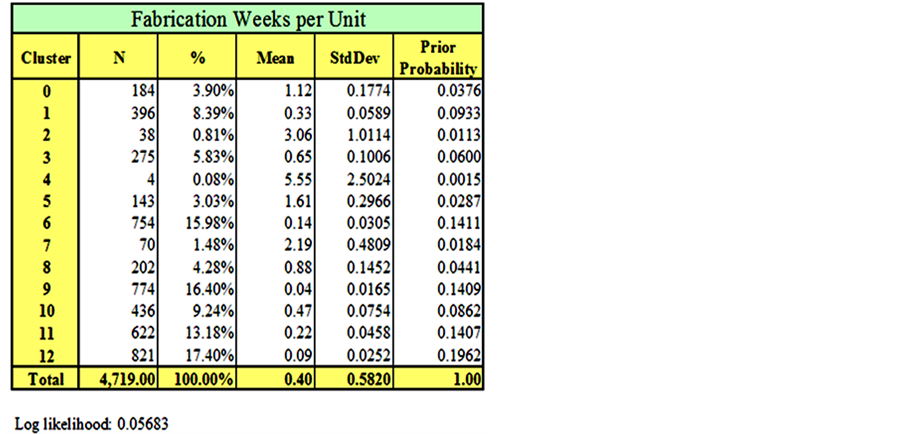
Figure 24. Clustering of fabrication weekly unit duration.
projects. These graphs show the required weekly hours of a specific resource within the duration of a project or work package. Data mining provides a set of various graphs based on different combinations of control attributes; hence, it provides contractors with the ability to utilize the most suitable graph. The current practices mostly rely on using uniform or predefined distribution graphs that do not rely on historical data and are not customized to reflect current conditions.
The third dataset to be used in this research was obtained from the same partner company that provided the first dataset. This third dataset contains the actual weekly hours for a set of resources per project phase. The current practice in the company is to collect actual hours by project phase instead of work packages. Although this data was not collected at the work package level as proposed in this research, this data is still very useful for providing analysis on the project level for providing Initial Planned Values (IPV) of project resource require-

Figure 25. Clustering of shop drawings’ hourly unit cost.

Figure 26. Clustering of shop drawings’ weekly unit duration.
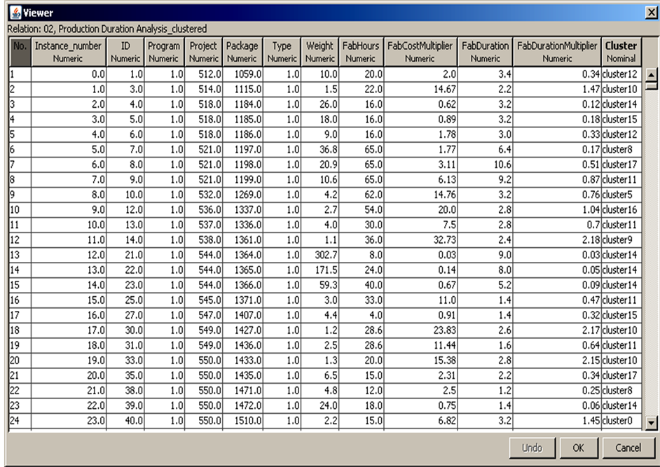
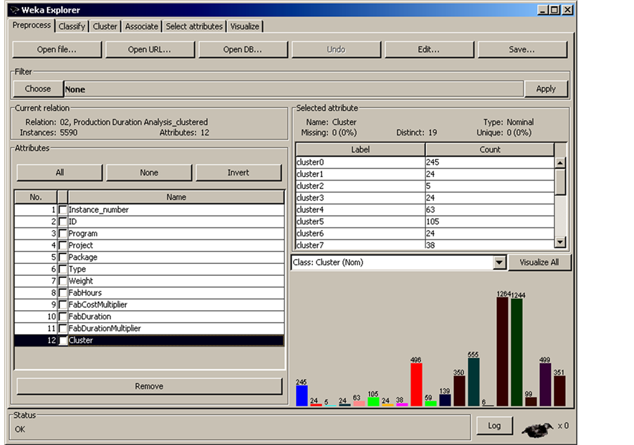
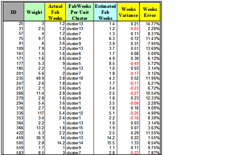
Figure 29. An excerpt of the validation tool for the fabrication phase.
ments. The same methodology can be applied to obtain resource utilization curves per work package for estimating resource requirements during the detailed planning stage of any project.
The procedure for obtaining the third dataset started with getting a list of all completed projects between the years 2004 and 2007, as shown in Figure 30. This list was obtained from the timekeeping system of the company, which is an in-house developed SQL server application. The list contained more than 1500 projects that vary in duration, cost and complexity. The data was automatically extracted out of the SQL-Server data tables to MS Excel for cleaning and preprocessing.
Project phase is an important control attribute for the data mining exercise. However, the company did not clearly assign project phases to the data points in their timekeeping system. As a result, it was necessary in this research to go back to the archives in order to assign the proper phase to each project. This process again consumed lots of time and effort.
Since the construction support phase is mostly responding to requests from sites and is not performed based on clearly defined scope, projects that were assigned to the "construction support" phase were eliminated from the dataset. Projects that were cancelled or put on hold prior to delivering their scope were eliminated from the list as well. At the end, there were more than 350 projects in the dataset. For each of these projects, a SQL statement was run to query the weekly working hours per resource type as shown in Figure 31.
The company did not store the original planned, current planned, earned hours on a weekly basis. Therefore, the missing data was simulated using random numbers in order to populate the data warehouse according to the proposed structure. The complete dataset was used to calculate the performance measures (CPI and SPI) on a weekly basis for all the data points.
The period end-date was used to calculate the week, month, quarter, and year numbers for each data point to expedite the procedure of running OLAP reports and queries. The formula used to calculate the year is:
 (6)
(6)
The formula used to calculate the month number is:
 (7)
(7)
The formula to calculate the week number is:
 (8)
(8)
The three-point sliding moving average was used to reduce the noise in the dataset [17]. After that, the duration data was normalized by dividing the week number by the total number of weeks. The cost data was also normalized by dividing the weekly hours by the total number of hours. The normalized data is shown in Figure 32.
Nassar [18] stated that dividing project progress to twenty equal periods with 5% increments is a very good method to measure project performance. Based on that, the dataset was normalized using the interpolation function of the R software.
As shown in Figure 33, each resource is now presents as an array R(1, 20). Each array is assigned to a single class. Each class represents a unique combination of a project phase, resource, size cluster and duration cluster. To obtain the size and duration clusters, the M-means clustering technique from Weka is used to classify the total resource of hours and project durations into groups. The clustering results are shown in Figures 34 and 35.
A dynamic program that allows using the polynomial regression to develop a function that represents the variation of resource utilization per week is developed in R. Polynomial regression is used when a relation between a dependent variable Y and independent variable X cannot be fit to a linear or curvilinear such as logarithmic (Log(X)), power (Xb) or exponential (bx) relationships, where b is a constant. As shown in the code below, the program reads the data from a Comma Separated Values (CSV) file and checks for the number of classes in the file.
After that, a cycle is used to transpose the data of each group and assign it in an array that can be recognized by the R software. For each array, the “Fit” function is used to obtain a polynomial regression function of the third degree that represents the data in each group. The function is in the format:
 (9)
(9)

Figure 30. List of completed projects between 2004 and 2007.
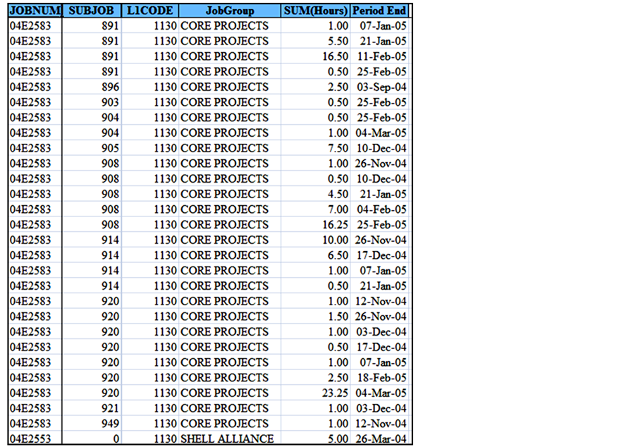
Figure 31. Weekly actual working hours per resource.
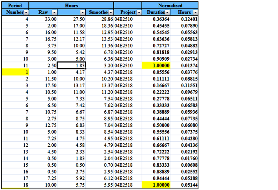
Figure 32. The normalized dataset.
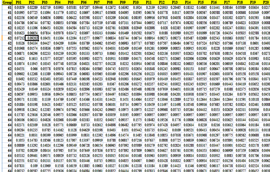
Figure 33. The normalized dataset after interpolation.

Figure 34. Clustering of total resource hours.

The third degree polynomial, sometimes referred to as cubic function, provides an S-curve, which fits reasonably well to the distribution of resource utilization over the project percent complete. The output of the developed code is a list of the coefficients: b0, b1, b2 and b3. The user can easily change the degree of the polynomial to any other degree using the function “PolDgr”. The goodness of fit is measured using the least square errors (R2) and the user can try different functions to find the one that fits best for the dataset under investigation.
The output of the code is written to another CSV file and an example of it is shown in Figure 36. The goodness of fit is tested using the R2 function and graphically. The output for each class is plotted accompanied with the original values of any class to visually test the goodness of fit. At the beginning of any internal project, the project can decide on the size and duration class for each resource, use the characteristics of these classes accompanied with the polynomial function for the distribution of these resource utilization over project percent complete to predict the initial planned values for each resource. These predicted values are based on PM judgment and historical data.
Another approach is to connect the averages of each percent complete (PI, P2 to P20). It is up to the user to decide on which methodology fits better for the existing data. This case study was used to provide the user with the Initial Planned Values (IPV) needed prior to the detailed planning of any project.
In the third dataset, project attributes were not clearly identified when data was collected. Moreover, some of the projects were not broken into clearly defined phases as proposed in this research. When data was analyzed, discrepancies were found among the resource utilization graphs. These discrepancies were highlighted and recommendations were made to the partner company.
5. Conclusion
5.1. Research Summary
The aim of this research was to improve resources management practices by using existing historical data from completed projects to forecast needs of future projects. During the process of managing labour resources in a multiple-project environment, a large amount of multidimensional data is generated, collected and stored in scattered formats. Currently, there is no consistent methodology to manage this wealth of data. Most of this data gets lost and is never viewed, analyzed or transferred to useful knowledge that could be an asset in improving resource management practices. This research developed an integrated framework for managing resources data in multiple-project environment. The framework is built on a KDD model to transfer the collected multidimensional historical data from completed projects to useful knowledge for new projects.
Three case studies were performed to validate the applicability of the developed framework to real projects data. The first dataset was obtained from a partner company and was utilized to define the distribution parame-
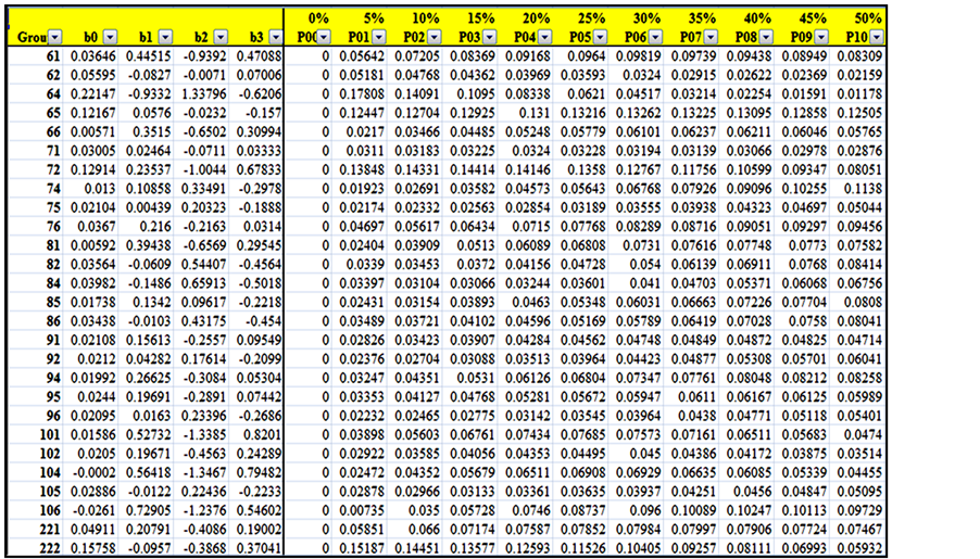
Figure 36. An example of the coefficients output.
ters of estimating unit costs. An anomaly detection methodology was developed to highlight the inconsistent data points for the end-user. A unit cost tree with branches was obtained. PostHoc tests and the One-way ANOVA were used to classify the cost units into a smaller number of groups. The second dataset was obtained from another partner company and was used to define the distribution parameters of estimating unit durations within different data clusters. The dataset was randomly divided into training set and testing set for validation purposes. More than 85% of the testing data points had an estimating error of less than 25%. The third dataset was used to analyze various resource utilization patterns over time units and to find the most fitting resources utilization curve per cluster.
By studying the original dataset, several problems were identified. These problems are mainly pertaining to the lack of a proper definition of data dimensions, objects and attributes and to the lack of a systematic consistent integrated approach to data collection and storage. There is a perception in the industry that each project is unique and its data is unique as well, and therefore, data from projects are not easily aggregated nor transferred to useful knowledge.
By implementing the data collection integrated framework to the original dataset, this research demonstrated that data can be collected in a systematic and consisted manner, which then could be analysed in a variety of ways, and then leads to extracting useful knowledge that would improve labour resources management practices and forecasts. As a result of this framework, productivity and efficiency would increase. As well, a continuous knowledge cycle and a self-learning loop would be established between completed and future projects.
5.2. Recommendations for Future Research
The developed KDD model was implemented into the management of labour resources data in industrial construction project domain. Further research can be carried out to investigate the feasibility of applying this model to other non-labour resources types. In addition, other researchers can investigate extending the application of this model to other domains such as infrastructure or commercial construction.
Clustering and anomaly detection data mining techniques were used to extract knowledge from the available datasets. Future research can apply other data mining techniques or knowledge discovery techniques such as classification, finding association rules, simulation, artificial neural networks, and fuzzy sets. The data warehouse would provide a systematic methodology to model projects, their objects and projects’ data for analysis by these sophisticated research methods.
Once populated with enough data, the data warehouse along with advanced research techniques can be used to identify the main factors impacting labour resources performance and overall project performance.
Acknowledgements
The authors would like to thank WorleyParsons Canada—Edmonton Division and Waiward Steel Fabricators Ltd. for providing the necessary data for the case study. This research was supported by the NSERC Industrial Research Chair in Construction Engineering and Management, IRCPJ 195558-10.
References
- Jergeas, G. (2008) Analysis of the Front-End Loading of Alberta Mega Oil Sands Projects. Project Management Journal, 39, 95-104. http://dx.doi.org/10.1002/pmj.20080
- Inmon, W.H. (2005) Building the Data Warehouse. Wiley, Indianapolis.
- Giovinazzo, W.A. (2000) Object-Oriented Data Warehouse Design: Building a Star Schema. Prentice Hall, Upper Saddle River.
- Ahmad, I., Azhar, S. and Lukauskis, P. (2004) Development of a Decision Support System Using Data Warehousing to Assist Builders/Developers in Site Selection. Automation in Construction, 13, 525-542. http://dx.doi.org/10.1016/j.autcon.2004.03.001
- Han, J. and Kamber, M. (2006) Data Mining: Concepts and Techniques. Morgan Kaufmann, Elsevier Science Distributor, San Francisco.
- Fayyad, U., Piatetsky-Shapiro, G. and Smyth, P. (1996) From Data Mining to Knowledge Discovery in Databases. AI Magazine, 17, 37.
- Cios, K.J. (2007) Data Mining: A Knowledge Discovery Approach. Springer, New York.
- Zaiane, O.R., Foss, A., Lee, C.H. and Wang, W. (2002) On Data Clustering Analysis: Scalability, Constraints, and Validation. Proceedings of the 6th Pacific-Asia Conference on Knowledge Discovery and Data Mining, Springer-Verlag, Berlin, 28-39.
- Soibelman, L. and Kim, H. (2002) Data Preparation Process for Construction Knowledge Generation through Knowledge Discovery in Databases. Journal of Computing in Civil Engineering, 16, 39-48. http://dx.doi.org/10.1061/(ASCE)0887-3801(2002)16:1(39)
- Chau, K.W., Cao, Y., Anson, M. and Zhang, J. (2002) Application of Data Warehouse and Decision Support System in Construction Management. Automation in Construction, 12, 213-224. http://dx.doi.org/10.1016/S0926-5805(02)00087-0
- Rujirayanyong, T. and Shi, J.J. (2006) A Project-Oriented Data Warehouse for Construction. Automation in Construction, 15, 800-807. http://dx.doi.org/10.1016/j.autcon.2005.11.001
- Moon, S.W., Kim, J.S. and Kwon, K.N. (2007) Effectiveness of OLAP-Based Cost Data Management in Construction Cost Estimate. Automation in Construction, 16, 336-344. http://dx.doi.org/10.1016/j.autcon.2006.07.008
- Fan, H., AbouRizk, S., Kim, H. and Zaiane, O. (2008) Assessing Residual Value of Heavy Construction Equipment Using Predictive Data Mining Model. Journal of Computing in Civil Engineering, 22, 181-191. http://dx.doi.org/10.1061/(ASCE)0887-3801(2008)22:3(181)
- Hammad, A., AbouRizk, S. and Mohamed, Y. (2013) Application of Knowledge Discovery in Data (KDD) Techniques to Extract Useful Knowledge from Labour Resources Data in Industrial Construction Projects. Journal of Management in Engineering. http://dx.doi.org/10.1061/(ASCE)ME.1943-5479.0000280
- Zaiane, O.R. (2006) Principles of Knowledge Discovery in Data. Lecture at University of Alberta. http://webdocs.cs.ualberta.ca/~zaiane/courses/cau/slides/cau-Lecture7.pdf
- Witten, I.H. and Frank, E. (2005) Data Mining: Practical Machine Learning Tools and Techniques. Morgan Kaufman, Amsterdam, Boston.
- Teicholz, P. (1993) Forecasting Final Cost and Budget of Construction Projects. Journal of Computing in Civil Engineering, 7, 511-529. http://dx.doi.org/10.1061/(ASCE)0887-3801(1993)7:4(511)
- Nassar, N.K. (2005) An Integrated Framework for Evaluation, Forecasting and Optimization of Performance of Construction Projects. PhD Thesis, University of Alberta (Canada), Canada.