Journal of Applied Mathematics and Physics
Vol.04 No.08(2016), Article ID:69478,60 pages
10.4236/jamp.2016.48147
Unified Field Theory
Ilija Barukčić
Internist, Horandstrasse, Jever, Germany

Copyright © 2016 by author and Scientific Research Publishing Inc.
This work is licensed under the Creative Commons Attribution International License (CC BY).
http://creativecommons.org/licenses/by/4.0/


Received 2 July 2016; accepted 1 August 2016; published 4 August 2016
ABSTRACT
In the Einstein field equations, the geometry or the curvature of space-time defined as depended on the distribution of mass and energy principally resides on the left-hand side is set identical to a non-geometrical tensorial representation of matter on the right-hand side. In one or another form, general relativity accords a direct geometrical significance only to the gravitational field while the other physical fields are not of space time. They reside only in space time. Less well known, though of comparable importance is Einstein’s dissatisfaction with the fundamental asymmetry between gravitational and non-gravitational fields and his contributions to develop a completely relativistic geometrical field theory of all fundamental interactions, a unified field theory. Of special note in this context and equally significant is Einstein’s demand to replace the symmetrical tensor field by a non-symmetrical one and to drop the condition gik = gki for the field components. Historically, many other attempts were made too, to extend the general theory of relativity’s geometrization of gravitation to non-gravitational interactions, in particular, to electromagnetism. Still, progress has been very slow. It is the purpose of this publication to provide a unified field theory in which the gravitational field, the electromagnetic field and other fields are only different components or ma- nifestations of the same unified field by mathematizing the relationship between cause and effect under conditions of general theory of relativity.
Keywords:
Quantum Theory, Relativity Theory, Unified Field Theory, Causality

1. Introduction
The historical development of physics as such shows that formerly unrelated and separated parts of physics can be fused into one single conceptual formalism. Maxwell’s theory unified the magnetic field and the electrical field once treated as fundamentally different. Einstein’s special relativity theory provided a unification of the laws of Newton’s mechanics and the laws of electromagnetism [1] . Thus far, the electromagnetic and weak nuclear forces have been unified together as an electroweak force. The unification with the strong interaction (chromodynamics) enabled the standard model of elementary particle physics. Meanwhile, the unification of gravitation with the other fundamental forces of nature is in the focus of much present research but still not in sight. A unification of all four fundamental interactions within one conceptual and formal framework has not yet met with success. Even Einstein himself spent years of his life on the unification [2] of the electromagnetic fields with the gravitational fields. In this context, Einstein’s position concerning the unified field theory is strict and clear (Figure 1).
Despite of the many and different approaches of theorists worldwide spanning so many of years taken to develop a unified field theory, to describe and to understand the nature at the most fundamental (quantum) level progress has been very slow. Thus far, a unification of all four fundamental interactions within one conceptual and formal framework has not yet met with success. Excellent and very detailed reviews, some of them in an highly and extraordinary satisfying way [3] , of the various aspects of the conceptually very different approaches of the unified field theories in the 20th century with a brief technical descriptions of the theories suggested and short biographical notes are far beyond the scope of this article and can be found in literature. The main focus of this article lies on the conceptual development of the geometrization of the electromagnetic field, by also paying attention to the unification of the electromagnetic and gravitational fields and the unified field theory as such. While the task to “geometrize” the electromagnetic field is not an easy one, a method how electromagnetic fields and gravitational fields can be joined into a new hyper-field [4] , will be developed, and a new common representation of all four fundamental interactions will be presented. As will be seen, with regard to unified field theories, formerly unrelated parts of physics will be fused into one single conceptual formalism while following a deductive-hypothetical approach. We briefly define and describe the basic mathematical objects and tensor calculus rules needed to achieve unification. In this context, the point of departure for a unified field theory will be in accordance with general relativity theory from the beginning. Still, in order to decrease the amount of notation needed, we shall restrict ourselves as much as possible to covariant second rank tensors.
Past experience has shown that formerly published papers with new theoretical perspectives should be based on a clear terminology thus that contradictions and misunderstandings are prevented from the beginning. The views in this paper are different in some instances. Thus far, this paper is written such that physicists should be able to follow the technical aspects of the papers without any problems, while philosophers of science and other reader without prior knowledge of the mathematics or of tensor calculus and general relativity at least might gain an insight into the new concepts, methods, and scientific background involved. As will be seen, with regard to new insights and conclusions, the rest of the paper is organized as follows. In the section, we will give some basic definitions and a terminological distinction. View of the immense amount of literature known theories will be covered only as much as is necessary for a better understanding of this paper. I apologize for the shortcoming. In all the attempts to develop some basic fundamental insights, I will encounter a deductive-hypothetical methodological approach. Especially in section theorems, the starting point of the theorems is axiom +1 = +1 (lex identitatis) which serves as common ground for quantum and relativity theory. The section discussion examines some conditions and consequences of the theorems proved.
2. Material and Methods
2.1. Definitions
2.1.1. Definition: The Pythagorean Theorem
The Pythagorean (or Pythagoras’) theorem is of far reaching and fundamental importance in Euclidean Geometry and in science as such. In physics, the Pythagorean (or Pythagoras’) theorem serves especially as a basis for the definition of distance between two points. Historically, it is difficult to claim with a great degree of credibility that Pythagoras (~560 - ~480 B.C.) or someone else from his School was the first to discover this theorem.

Figure 1. Einstein and the problem of the unified field theory.
There is some evidence, that the Pythagorean (or Pythagoras’) theorem was discovered on a Babylonian tablet [5] circa 1900 - 1600 B.C. Meanwhile, there are more than 100 published approaches proving this theorem, probably the most famous of all proofs of the Pythagorean proposition is the first of Euclid's two proofs (I.47), generally known as the Bride’s Chair. The Pythagorean (or Pythagoras’) theorem states that the sum of (the areas of) the two small squares equals (the area of) the big one square. In algebraic terms we obtain
 (1)
(1)
where c represents the length of the hypotenuse (the longest side within a right angled triangle) and a and b represents the lengths of the triangle’s other two sides or legs (or catheti, singular: cathetus, greek: káthetos). Following Euclid (Elements Book I, Proposition 47) in right-angled triangles the sum of the squares on the sides containing the right angle equals the square on the side opposite the right angle.
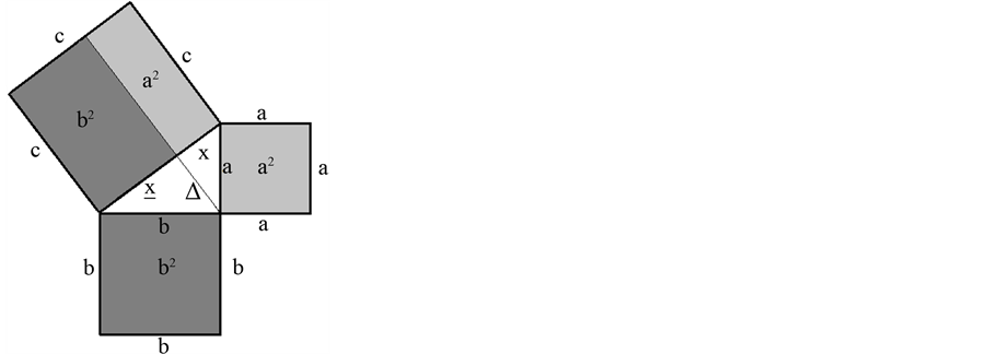
2.1.2. Definition: The Normalization of the Pythagorean Theorem
The normalization of the Pythagorean theorem is defined as
 (2)
(2)
where c represents the length of the hypotenuse (the longest side within a right angled triangle) and a and b represents the lengths of the triangle’s other two sides/legs.
2.1.3. Definition: The Negation Due to the Pythagorean Theorem
We define the negation of x, denoted as n(x), as
 (3)
(3)
We define the negation of anti x, denoted as n(x), as
 (4)
(4)
In general, it is
 (5)
(5)
2.1.4. Definition: The Determination of the Hypotenuse of a Right Angled Triangle
In general, we define
 (6)
(6)
where x and x denotes the segments on the hypotenuse c of a right angled triangle (c is the longest side within a right angled triangle).
Scholium.
Form this follows that (C × X) + (C × X) = C². Due to our definition above, it is (C × X) = a² and b² = (C × X). The Pythagorean theorem is valid even if x = 1 and x = +∞ −1 while c = +∞. Under these assumptions, the Pythagorean theorem is of use to prove the validity of the claim that +1/+0 = +∞. In general, the normalized form of negation is denoted as (1 −).
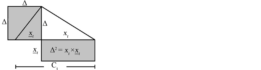
2.1.5. Definition: The Euclid’s Theorem
According to Euclid’s (ca. 360 - 280 BC) so called geometric mean theorem or right triangle altitude theorem or Euclid’s theorem, published in Euclid’s Elements in a corollary to proposition 8 in Book VI, used in proposition 14 of Book II [6] to square a rectangle too, it is
 (7)
(7)
where Δ denotes the altitude in a right triangle and x and x denote the segments on the hypotenuse c of a right angled triangle.
Scholium.
The variance of a right angled triangle, denoted as s(x)², can be defined as
 (8)
(8)
where Δ denotes the altitude in a right triangle and x and x denote the segments on the hypotenuse c of a right angled triangle.
2.1.6. Definition: The Gradient
The gradient, denoted as grad(a, b), a measure of how steep a slope or a line is, is defined by dividing the vertical height a by the horizontal distance b of a right angled triangle. In other words, we obtain
 (9)
(9)
Scholium.
The following picture of a right angled triangle may illustrate the background of a gradient
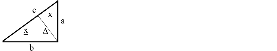
where b denotes the run; a denotes the rise and c denotes the slope length. The gradient has several meanings. In mathematics, the gradient is more or less something like a generalization of a derivative of a function in one dimension to a function in several dimensions. Consider a n-dimensional manifold with coordinates 1x, 2x, nx. The gradient of a function f(1x, 2x, nx) is defined as
 (10)
(10)
Due to our definition above it is equally c² ´ n(x) = a². In this case c² is not identical to the speed of the light but with the hypotenuse, the longest side within a right angled triangle. Equally, it is c² ´ n(x) = b². In general, it is true that . The raise can be calculated as
 . In other words, it is a/b = y ´ (x/c) or
 .
.
2.2. Einstein’s Special Theory of Relativity
2.2.1. Definition: The Relativistic Energy RE (of a System)
In general, it is
 (11)
(11)
where RE denotes the total (“relativistic”) energy of a system; Rm denotes the “relativistic” mass and c denotes the speed of the light in vacuum.
Scholium.
Einstein defined the matter/mass-energy equivalence as follows:
“Gibt ein Körper die Energie L in Form von Strahlung ab, so verkleinert sich seine Masse um L/V² … Die Masse eines Körpers ist ein Maß für dessen Energieinhalt” [7] .
In other words, due to Einstein, energy and mass are equivalent.
“Eines der wichtigsten Resultate der Relativitätstheorie ist die Erkenntnis, daß jegliche Energie E eine ihr proportionale Trägheit (E/c²) besitzt” [8] .
It was equally correct by Einstein to point out that matter/mass and energy are equivalent.
“Da Masse und Energie nach den Ergebnissen der speziellen Relativitätstheorie das Gleiche sind und die Energie formal durch den symmetrischen Energietensor (Tµv) beschrieben wird, so besagt dies, daß das G-Geld [gravitational field, author] durch den Energietensor der Materie bedingt und bestimmt ist” [9] .
The term relativistic mass Rm was coined by Gilbert and Tolman [10] .
2.2.2. Definition: Einstein’s Mass-Energy Equivalence Relation
The Einsteinian matter/mass-energy equivalence [7] lies at the core of today physics. In general, due to Einstein’s special theory of relativity it is
 (12)
(12)
or equally
 (13)
(13)
or equally
 (14)
(14)
where OE denotes the “rest” energy; Om denotes the “rest” mass; RE denotes the “relativistic” energy; Rm denotes the “relativistic” mass; v denotes the relative velocity between the two observers and c denotes the speed of light in vacuum.
2.2.3. Definition: Normalized Relativistic Energy-Momentum Relation
The normalized relativistic energy momentum relation [10] , a probability theory consistent formulation of Einstein’s energy momentum relation, is determined as
 (15)
(15)
while the “particle-wave-dualism” [10] is determined as
 (16)
(16)
where WE = (Rp ´ c) denotes the energy of an electro-magnetic wave and Rp denotes the “relativistic” momentum while c is the speed of the light in vacuum.
2.2.4. Definition: The Relativistic Potential Energy
Following Einstein in his path of thoughts, we define the relativistic potential energy pE [11] as
 (17)
(17)
Scholium.
The definition of the relativistic potential energy pE is supported by Einstein’s publication in 1907. Einstein himself demands that there is something like a relativistic potential energy.
“Jeglicher Energie E kommt also im Gravitationsfelde eine Energie der Lage zu, die ebenso groß ist, wie die Energie der Lage einer ‘ponderablen’ Masse von der Größe E/c²” [12] .
Translated into English:
“Thus, to each energy E in the gravitational field there corresponds an energy of position that equals the potential energy of a ‘ponderable’ mass of magnitude E/c²”.
The relativistic potential energy pE can be viewed as the energy which is determined by an observer P which is at rest relative to the relativistic potential energy. The observer which is at rest relative to the relativistic potential energy will measure its own time, the relativistic potential time pt.
2.2.5. Definition: The Relativistic Kinetic Energy (the “Vis Viva”)
The relativistic kinetic energy KE is defined [10] in general as
 (18)
(18)
where Rm denotes the “relativistic mass” and v denotes the relative velocity. In general, it is
 (19)
(19)
where PE denotes the relativistic potential energy; KE denotes the relativistic kinetic energy; PH denotes the Hamiltonian of the relativistic potential energy; KH denotes the Hamiltonian of the relativistic kinetic energy. Multiplying this equation by the wave function RY, we obtain relativity consistent form of Schrödinger’s equation as
 (20)
(20)
Scholium.
The historical background of the relativistic kinetic energy KE is back grounded by the long lasting and very famous dispute between Leibniz (1646-1716) and Newton (1642-1726). In fact, the core of this controversy was the dispute about the question, what is preserved through changes. Leibnitz himself claimed, that “vis viva” [13] , [14] or the relativistic kinetic energy KE = Rm × v × v was preserved through changes. In contrast to Leibnitz, Newton was of the opinion that the momentum Rp = Rm × v was preserved through changes. The observer which is at rest relative to the relativistic kinetic energy will measure its own time, the relativistic kinetic time kt.
2.2.6. Definition: Einstein’s Relativistic Time Dilation Relation
An accurate clock in motion slows down with respect a stationary observer (observer at rest). The proper time Ot of a clock moving at constant velocity v is related to a stationary observer’s coordinate time Rt by Einstein’s relativistic time dilation [15] and defined as
 (21)
(21)
where Ot denotes the “proper” time; Rt denotes the “relativistic” (i.e. stationary or coordinate) time; v denotes the relative velocity and c denotes the speed of light in vacuum.
Scholium.
Coordinate systems can be chosen freely, deepening upon circumstances. In many coordinate systems, an event can be specified by one time coordinate and three spatial coordinates. The time as specified by the time coordinate is denoted as coordinate time. Coordinate time is distinguished from proper time. The concept of proper time, introduced by Hermann Minkowski in 1908 and denoted as Ot, incorporates Einstein’s time dilation effect. In principle, Einstein is defining time exclusively for every place where a watch, measuring this time, is located.
“… Definition … der … Zeit … für den Ort, an welchem sich die Uhr … befindet…” [15] .
In general, a watch is treated as being at rest relative to the place, where the same watch is located.
“Es werde ferner mittels der imruhenden System befindlichen ruhenden Uhren die Zeit t [i.e. Rt, author] des ruhenden Systems … bestimmt, ebenso werde die Zeit t [Ot, author] des bewegten Systems, in welchen sich relativ zu letzterem ruhende Uhren befinden, bestimmt…” [15] .
Due to Einstein, it is necessary to distinguish between clocks as such which are qualified to mark the time Rt when at rest relatively to the stationary system R, and the time Ot when at rest relatively to the moving system O.
“Wir denken uns ferner eine der Uhren, welche relativ zum ruhenden System ruhend die Zeit t [Rt, author], relativ zum bewegten System ruhend die Zeit t [Ot, author] anzugeben befähigt sind…” [15] .
In other words, we have to take into account that both clocks i.e. observers have at least one point in common, the stationary observer R and the moving observer O are at rest, but at rest relative to what? The stationary observer R is at rest relative to a stationary co-ordinate system R, the moving observer O is at rest relative to a moving co-ordinate system O. Both co-ordinate systems can but must not be at rest relative to each other. The time Rt of the stationary system R is determined by clocks which are at rest relatively to that stationary system R. Similarly, the time Ot of the moving system O is determined by clocks which are at rest relatively to that the moving system O. In last consequence, due to Einstein’s theory of special relativity, a moving clock (Ot) will measure a smaller elapsed time between two events than a non-moving (inertial) clock (Rt) between the same two events.
2.2.7. Definition: The Normalized Relativistic Time Dilation Relation
As defined above, due to Einstein’s special relativity, it is
 (22)
(22)
where Ot denotes the “proper” time, Rt denotes the “relativistic” (i.e. stationary or coordinate) time, v denotes the relative velocity and c denotes the speed of light in vacuum. Equally, it is
 (23)
(23)
or
 (24)
(24)
or
 (25)
(25)
The normalized relativistic time dilation is defined as
 (26)
(26)
In general, under conditions of the special theory of relativity, we define
 (27)
(27)
and
 (28)
(28)
and
 (29)
(29)
Scholium.
The following 2 × 2 table may illustrate the relationships before (Table 1).
The causal relationship k [16] under conditions of special theory of relativity (i.e. the particle-production apparatus) follows as
 (30)
(30)
Under conditions [17] where
 (31)
(31)
there is a relationship between the causal relationship k the Schrödinger equation in the form
 (32)
(32)
2.3. Einstein’s General Theory of Relativity
2.3.1. Definition: The General Kronecker Delta
The general Kronecker delta dmn, named after Leopold Kronecker, is +1 if the variables m and n are equal, and +0 otherwise.
Scholium.
For convenience, the restriction to positive integers is common, but not necessary. The general Kronecker delta, running from 1 to 4, denoted as dmn can be displayed in matrix form as
 (33)
(33)
The anti general Kronecker delta denoted as dmn is defined as .
.
2.3.2. Definition: The Special Kroneker Delta
The special Kronecker delta d(i, j)mn, named after Leopold Kronecker, is +1 if and only if m = i and if n = j and +0 otherwise.

Table 1. The unified field under conditions of the special theory of relativity.
Scholium.
Example. The special Kronecker delta  for
for  and
and , running from 1 to 4, can be displayed in matrix form as
 (34)
(34)
The anti special Kronecker delta denoted as d(i, j)mn and defined as  for
for  and
and , running from 1 to 4, can be displayed as
 (35)
(35)
The special Kronecker delta is not grounded on the equality that m = n but on the fact, the m equal to a certain value i and that n is equal to another certain value j. In other words, it is m = i and n = j.
2.3.3. Definition: The Metric Tensor gµv
In the following, let us define the following. Let
 (36)
(36)
and
 (37)
(37)
In Euclidean coordinates for an n-dimensional space the formula for the length ds² of an infinitesimal line segment due to the Pythagorean theorem follows as
 (38)
(38)

or
 (39)
(39)
In general, a coordinate system can be changed from the Euclidean X’s to some coordinate system of Y’s then
 (40)
(40)
and
 (41)
(41)
The Pythagorean theorem is defined as
 (42)
(42)
While using Einstein’s summation convention, a (i.e. position dependent) metric tensor g(x)µv is defined as
 (43)
(43)
and a curved space compatible formulation of the Pythagorean theorem follows as
 (44)
(44)
Scholium.
The metric tensor generalizes the Pythagorean theorem of flat space in a manifold with curvature. The metric tensor can be decomposed in many different ways. Let gµv = nµv + nµv where gµv is the metric tensor of general relativity; nµv is the tensor of special relativity and nµv is the anti tensor of general relativity. In general theory of relativity, the scalar Newtonian gravitational potential is replaced by the metric tensor. “In particular, in general realtivity, the gravitational potential is replaced by the metric tensor gab” [18] . In last consequence, the gravitational potential is something like a feature of the metric tensor. Following Renn et al., the metric tensor is “… the mathematical representation of the gravitation alpotential…” [19] . On this account it is necessary to make a distinction between a gravitational potential and a gravitational field. Due to Einstein, “… the introduction of independent gravitational fields is considered justified even though no masses generating the field are defined” [2] . The question is, can a gravitational potential exist even though no masses generating the gravitational potential are defined?
2.3.4. Definition: The Normalized Metric Tensor n(X)µv
In the following, we define the normalized metric tensor nµv, while using Einstein’s summation convention, as
 (45)
(45)
The line element follows in general as
 (46)
(46)
Scholium.
The normalized metric tensor is not based on the gradient. The metric tensor passes over into the normalized metric tensor and vice versa. We obtain
 (47)
(47)
or
 (48)
(48)
2.3.5. Definition: Einstein’s Field Equations
Einstein field equations (EFE), originally [20] published [21] without the extra “cosmological” term Λ ´ gµv [22] may be written in the form
 (49)
(49)
where Gµv is the Einsteinian tensor; Tµv is the stress-energy tensor of matter (still a field devoid of any geometrical significance); Rµv denotes the Ricci tensor (the curvature of space); R denotes the Ricci scalar (the trace of the Ricci tensor); Λ denotes the cosmological “constant” and gµv denotes the metric tensor (a 4 × 4 matrix) and where p is Archimedes’ constant (p = 3.1415926535897932384626433832795028841971693993751058209…) and g is Newton’s gravitational “constant” and the speed of light in vacuum is c = 299,792,458 [m/s] in S. I. units.
Scholium.
The stress-energy tensor Tµv, still a tensor devoid of any geometrical significance, contains all forms of energy and momentum which includes all matter present but of course any electromagnetic radiation too. Originally, Einstein’s universe was spatially closed and finite. In 1917, Albert Einstein modified his own field equations and inserted the cosmological constant Λ (denoted by the Greek capital letter lambda) into his theory of general relativity in order to force his field equations to predict a stationary universe.
“Ich komme nämlich zu der Meinung, daß die von mir bisher vertretenen Feldgleichungen der Gravitation noch einer kleinen Modifikation bedürfen…” [22] .
By the time, it became clear that the universe was expanding instead of being static and Einstein abandoned the cosmological constant Λ. “Historically the term containing the ‘cosmological constant’ l was introduced into the field equations in order to enable us to account theoretically for the existence of a finite mean density in a static universe. It now appears that in the dynamical case this end can be reached without the introduction of l” [23] . But lately, Einstein’s cosmological constant is revived by scientists to explain a mysterious force counteracting gravity called dark energy. In this context it is important to note that Newton’s gravitational “constant” big G is not [24] [25] a constant.
2.3.6. Definition: General Tensors
Independently of the tensors of the theory of general relativity, we introduce by definition the following covariant second rank tensors of yet unknown structure whose properties we leave undetermined as well. We define the following covariant second rank tensors of yet unknown structure as
 (50)
(50)
Tensor can be decomposed (sometimes in many different ways). In the following of this publication we define the following relationships. It is
 (51)
(51)
 (52)
(52)
 (53)
(53)
 (54)
(54)
 (55)
(55)
Scholium.
The following 2 × 2 table may illustrate the relationships above (Table 2).
These tensors above may have different meanings depending upon circumstances. The unified field RWµv can be decomposed into several (sub-) fields Aµv, Bµv, Cµv, Dµv. In order to achieve unification between general relativity theory and quantum (field) theory the (sub-) fields Aµv, Bµv, Cµv, Dµv can denote the four basic fields of nature. The idea of quantum field theory is to describe a particle as a manifestation of an abstract field. In this context the particle ai can be associated with the field Aµv, the particle bi can be associated with the field Bµv, the particle ci can be associated with the field Cµv, the particle di can be associated with the field Dµv. Thus far, we can define something like Aµv = ai × FAµv and Bµv = bi × FBµv and Cµv = ci × FCµv and Dµv = di × FDµv where the subscript F can denote an individual particle field. Under conditions of general relativity, Einstein field equation can be rewritten (using the tensors above) as
Table 2. The unified field RWµv.
 (56)
(56)
where  and
and . From an epistemological point of view
 is the tensor of the cause (in German: Ursache U) while
  is the tensor of the effect (in German: Wirkung W). As we will see, from the definition
  follows that
 even if Einstein’s cosmological constant Λ cannot [26] be treated as a constant.
2.4. Unified Field Theory
2.4.1. Definition: The Tensor of Planck’s Constant h
Planck defined in 1901 the constant of proportionality [27] as h. As long as Planck’s constant h is a constant, a tensor form of this constant is not needed. We define the co-variant second rank tensor of Planck’s constant Rhµv as
 (57)
(57)
2.4.2. Definition: The Tensor of Dirac’s Constant
We define the co-variant second rank tensor of Dirac’s constant as
 (58)
(58)
Scholium.
In general it is known that
 (59)
(59)
2.4.3. Definition: The Tensor of Speed of the Light Rcµv
We define the co-variant second rank tensor of the speed of the light Rcµv, denoted by small letter c, as
 (60)
(60)
where Rfµv denotes the stress energy tensor of frequency and Rlµv denotes the wave-length tensor.
Scholium.
Following Einstein’s own position, the constancy of the speed of the light c is something relative and nothing absolute. Theoretically, circumstances are possible where the speed of the light is not constant. Einstein himself linked the constancy of the speed of the light c to a constant gravitational potential.
“Dagegen bin ich der Ansicht, daß das Prinzip der Konstanz der Lichtgeschwindigkeit sich nur insoweit aufrecht erhalten läßt, als man sich auf raum-zeitliche Gebiete von konstantem Gravitationspotential beschränkt. Hier liegt nach meiner Meinung die Grenze der Gültigkeit … des Prinzips der Konstanz der Lichtgeschwin- digkeit und damit unserer heutigen Relativitätstheorie” [8] .
Thus far a tensor of the speed of the light is of use to face these theoretical possibilities.
2.4.4. Definition: The Tensor of Newton’s Gravitational “Constant” Rgµv
We define the co-variant second rank tensor of Newton’s gravitational constant Rgµv as
 (61)
(61)
Scholium.
Newton’s gravitational constant is not for sure a constant. Therefore, we prefer to use the same in the form of a tensor.
2.4.5. Definition: The Tensor of Archimedes “Constant” Rpµv
We define the co-variant second rank tensor of Archimedes constant Rpµv as
 (62)
(62)
Scholium.
Archimedes of Syracuse (ca. 287 BC - ca. 212 BC) himself was able to find p, the circumference of a circle with diameter 1 commonly approximated as 3.14159, to 99.9% accuracy about 2000 years ago. Archimedes constant p is an irrational number, p never settles into a permanent repeating pattern, the decimal representation of Archimedes constant p never ends.
2.4.6. Definition: The Tensor of Imaginary Number iµv
We define the co-variant second rank tensor of the imaginary number iµv as
 (63)
(63)
2.4.7. Definition: The Tensor of Space
We define the second rank tensor of space of yet unknown structure as
 (64)
(64)
Under conditions of general relativity, we define
 (65)
(65)
where Rµv denotes the Ricci tensor, the tensor of the curvature of space. Under conditions different form general relativity, RSµv can be determined in a different way. It is important to note that RUµv is not identical with Uµv.
2.4.8. Definition: The Tensor of Energy
Similar to general theory of relativity, it is at present appropriate to introduce a corresponding energy tensor, a tensor which represents the amounts of energy, momentum, pressure, stress et cetera in the space, a tensor which describes the energy/matter/momentum et cetera distribution (at each event) in space. The energy tensor expressed mathematically by a symmetrical tensor of the second rank of yet unknown structure is defined as
 (66)
(66)
Ipso facto, the same tensor is determined by all matter present but of course any electromagnetic radiation too. Under conditions of general relativity, we define
 (67)
(67)
To assure compatibility with quantum theory, we define
 (68)
(68)
Due to the definition before we obtain
 (69)
(69)
The tensor of probability of energy follows as
 (70)
(70)
General relativity’s geometry of space and time is one but not the only one geometry of space and time. Especially general relativity’s stress-energy tensor as the source-term of Einstein’s field equations is still a field devoid of any geometrical significance. A geometrical tensorial representation of the stress energy tensor of energy is possible as
 (71)
(71)
2.4.9. Definition: The Tensor of Frequency
In general, we define the covariant second rank tensor of frequency Rfµv as
 (72)
(72)
To assure compatibility with quantum theory, we define the inverse tensor Rtµv of the covariant second rank tensor of frequency Rfµv as
 (73)
(73)
Per definition it follows that
 (74)
(74)
2.4.10. Definition: The Tensor 0wµv
In general, we define the covariant second rank tensor 0wµv as
 (75)
(75)
Scholium.
The tensor of frequency Rfµv and the 0wµv tensor are related. Under circumstances of general relativity, there are conditions where
 (76)
(76)
2.4.11. Definition: The Tensor of Matter RMµv
The matter tensor expressed mathematically by a symmetrical tensor of the second rank of yet unknown structure is defined as
 (77)
(77)
Under conditions of general relativity, we define
 (78)
(78)
Scholium.
This definition is based on the equivalence of mass/matter and energy due to Einstein’s special theory of relativity.
“Da Masse und Energie nach den Ergebnissen der speziellen Relativitätstheorie das Gleiche sind und die Energie formal durch den symmetrischen Energietensor (Tµv) beschrieben wird, so besagt dies, daß das G-Geld [gravitational field, author] durch den Energietensor der Materie bedingt und bestimmt ist” [9] .
2.4.12. Definition: The Tensor of Ordinary Energy 0Eµv
We define the second rank tensor of ordinary energy 0Eµv of yet unknown structure as
 (79)
(79)
Scholium.
Under some well defined circumstances, 0Eµv can denote the unity of strong interaction and weak interaction. Under conditions of general relativity, it is
 (80)
(80)
The associated probability tensor can be achieved as
 (81)
(81)
2.4.13. Definition: The Tensor of “Ordinary” Matter 0Mµv
The tensor of ordinary mater expressed mathematically as a covariant second rank of yet unknown structure is defined as
 (82)
(82)
2.4.14. Definition: The Anti Tensor of “Ordinary” Matter 0Eµv
We define the second rank anti tensor 0Eµv of the tensor 0Eµv as
 (83)
(83)
Under conditions of general relativity, where 0Eµv is tensor of ordinary energy/matter, the electromagnetic field is an anti tensor of ordinary energy/matter. Under conditions of general relativity, the tensor of the electromagnetic field is determined by an anti-symmetric second-order tensor known as the electromagnetic field (Faraday) tensor F. In general, under conditions of general relativity, the second rank covariant tensor of the electromagnetic field in the absence of “ordinary” matter, which is different from the electromagnetic field tensor F, is defined by
 (84)
(84)
where F is the electromagnetic field tensor and gµv is the metric tensor.
Scholium.
The associated probability tensor is determined as
 (85)
(85)
The geometric formulation of the stress-energy tensor of the electromagnetic field follows as
 (86)
(86)
2.4.15. Definition: The Tensor 0Mµv
The tensor 0Mµv is defined as
 (87)
(87)
2.4.16. Definition: The Decomposition of the Tensor of Energy
A portion of the tensor of energy is due to the tensor of the electromagnetic field, another portion of the tensor of energy is due to the tensor of ordinary energy. Before going on to discuss this topic in more detail, we define in general
 (88)
(88)
Under conditions of general relativity, we define
 (89)
(89)
Scholium.
The stress-energy tensor of the electromagnetic field is equivalent to the portion of the stress-energy tensor of energy due to the electromagnetic field. In this approach, we are following Vranceanu in his position, that the energy tensor Tkl can be treated as the sum of two tensors one of which is due to the electromagnetic field.
“On peut aussi supposer que le tenseur d’énergie Tkl soit la somme de deux tenseurs dont un dû au champ électromagnétique…” [28] .
In English:
“One can also assume that the energy tensor Tkl be the sum of two tensors one of which is due to the electromagnetic field”.
Einstein himself demanded something similar.
“Wir unterscheiden im folgenden zwischen ‘Gravitationsfeld’ und ‘Materie’ in dem Sinne, daß alles außer dem Gravitationsfeld als ‘Materie’ bezeichnet wird, also nicht nur die ‘Materie’ im üblichen Sinne, sondern auch das elektromagnetische Feld” [21] .
2.4.17. Definition: The Tensor of Time Rtµv
We define the second rank tensor of time of yet unknown structure as
 (90)
(90)
Scholium.
All but energy is time, there is no third between energy and time. Under conditions of general theory of relativity, the associated probability tensor follows as
 (91)
(91)
2.4.18. Definition: The Tensor Rgµv
We define the second rank tensor Rgµv as
 (92)
(92)
Scholium.
The tensor
 (93)
(93)
is not identical with the metric tensor of general relativity, defined as
 (94)
(94)
Still, circumstances may exist, where both tensors can be treated as being identical.
2.4.19. Definition: The Tensor 0tµv
We define the second rank tensor 0tµv as
 (95)
(95)
Scholium.
Under conditions of general theory of relativity, the associated probability tensor follows as
 (96)
(96)
2.4.20. Definition: The Tensor 0gµv
We define the second rank tensor 0gµv as
 (97)
(97)
2.4.21. Definition: The Tensor Wtµv
We define the second rank tensor Wtµv as
 (98)
(98)
Scholium.
Under conditions of general theory of relativity, the associated probability tensor follows as
 (99)
(99)
2.4.22. Definition: The Tensor Wgµv
We define the second rank tensor Wgµv as
 (100)
(100)
2.4.23. Definition: The Wave Function Tensor RYµv
We define the covariant second rank wave function tensor as
 (101)
(101)
Under conditions of general relativity, we define
 (102)
(102)
2.4.24. Definition: The Complex Conjugate Wave Function Tensor R*Yµv
We define the covariant second rank complex conjugate wave function tensor of yet unknown structure as
 (103)
(103)
2.4.25. Definition: The Decomposition of the Tensor of Space
A portion of the tensor of space is due to the tensor of time, another portion of the tensor of space is determined by the tensor of energy. In general, we define
 (104)
(104)
The field equation of the unified field theory follows in general as
 (105)
(105)
where RSµv denotes the tensor of space; REµv denotes the tensor of energy and Rtµv denotes the tensor of time.
2.4.26. Definition: The Normalization of the Tensor of Space
Let RYµv denote a covariant second rank tensor of preliminary unknown structure. In general, we define
 (106)
(106)
Scholium.
In general, the properties of the tensor RYµv are unknown. But one property of this tensor is known and this property assures the normalisation of the tensor of space as RSµv Ç RYµv = 1µv. Under conditions of the general theory of relativity, it is true that as RSµv = Rµv and we do obtain Rµv Ç RYµv = 1µv.
2.4.27. Definition: The Probability Tensor
Let
 (107)
(107)
denote a covariant second rank probability tensor of yet unknown structure as associated with a tensor RXµv. The probability tensor p(RYµv) of yet unknown structure as associated with the wave function tensor RYµv is defined as
 (108)
(108)
2.4.28. Definition: General Covariant form of Born’s Rule
Under the assumption of the validity of Born’s rule even under conditions of accelerated frames of reference, we define
 (109)
(109)
where p(RYµv) denotes the probability tensor as associated i.e. with the wave function tensor RYµv and  is the covariant second rank complex conjugate wave function tensor and Ç denotes the commutative multiplication of tensors.
2.4.29. Definition: The Probability Tensor II
In general, we define
 (110)
(110)
where p(RYµv) denotes the probability tensor as associated i.e. with the wave function tensor RYµv and RYµv denote a covariant second rank tensor of preliminary unknown structure and Ç denotes the commutative multiplication of tensors.
Scholium.
The properties of the tensor RYµv, as mentioned already before, are still unknown. Still, another second property of this tensor is the special relationship with the wave function tensor RYµv. The interaction of the tensor RYµv with the wave function tensor RYµv yields the probability tensor p(RYµv) as associated with the wave function tensor RYµv. In general it is p(RYµv) = RYµv Ç RYµv.
2.4.30. Definition: The Tensor Uµv
In general, we define the tensor Uµv of yet unknown structure as
 (111)
(111)
2.4.31. Definition: The Decomposition of the Tensor Uµv
In general, we decompose the tensor Uµv as
 (112)
(112)
Scholium.
By this definition we are following Einstein in his claim that something is determined by matter and the gravitational field. In other words, there is no third between matter and gravitational field, i.e. all but matter is gravitational field. To proceed further, in following Einstein, we make a strict distinction between matter and gravitational field too.
“Wir unterscheiden im folgenden zwischen ‘Gravitationsfeld’ und ‘Materie’ in dem Sinne, daß alles außer dem Gravitationsfeld als ‘Materie’ bezeichnet wird, also nicht nur die ‘Materie’ im üblichen Sinne, sondern auch das elektromagnetische Feld” [21] .
The tensor RUµv is not identical with the tensor Uµv. In terms of set theory, we do obtain the following picture (Table 3).
2.4.32. Definition: The Tensor of Curvature 0Cµv
In general, we define the tensor of curvature as 0Cµv of yet unknown structure as
 (113)
(113)
where Gµv is the Einsteinian tensor; Rµv is the Ricci tensor; R is the Ricci scalar and gµv is the metric tensor of general relativity. Under conditions of the theory of general relativity it is 0Cµv = Gµv.
Scholium.
Table 3. The relationship between matter and gravitational field.
Under conditions of general theory of relativity, the associated probability tensor follows as
 (114)
(114)
2.4.33. Definition: The Tensor of Anti-Curvature 0Cµv
In general, we define the tensor of anti-curvature as 0Cµv of yet unknown structure as
 (115)
(115)
where RSµv is the tensor of space, 0Cµv is the tensor of curvature. Under conditions of general relativity, the tensor of anti-curvature is equivalent with
 (116)
(116)
where Gµv is the Einsteinian tensor; Rµv is the Ricci tensor; R is the Ricci scalar and gµv is the metric tensor of general relativity.
Scholium.
Under conditions of general theory of relativity, the associated probability tensor follows as
 (117)
(117)
2.5. Tensor Calculus
2.5.1. Definition: The Tensor of the Unified Field 1µv
In general, we define the tensor of the unified field 1µv, as
 (118)
(118)
Scholium.
Every component of the tensor of the unified field is equal to +1. The tensor of the unified field is of order two, its components can be displayed in 4 × 4 matrix form as
 (119)
(119)
2.5.2. Definition: The Zero Tensor 0µv
In general, we define the zero tensor 0µv as
 (120)
(120)
Scholium.
Every component of a zero tensor is equal to +0. The zero tensor is of order two, its components can be displayed in 4 × 4 matrix form too as
 (121)
(121)
2.5.3. Definition: The Tensor of the Number 2µv
In general, we define tensor of any number, i.e. the number 2µv as
 (122)
(122)
Scholium.
Every component of a tensor of the number +2 is equal to +2. The tensor of the number +2 can be displayed in 4 × 4 matrix form as
 (123)
(123)
2.5.4. Definition: The Tensor of Infinity ∞µv
In general, we define the tensor of infinity ∞µv as
 (124)
(124)
Scholium.
Every component of the tensor of infinity is equal to +∞. The tensor of infinity is of order two, its components can be displayed in 4 × 4 matrix form as
 (125)
(125)
2.5.5. Definition: The Symmetrical Part of a Tensor S(0Xµv)
Let 0Xµv denote a second-tensor rank. The symmetric part of a tensor 0Xµv is defined as
 (126)
(126)
and denoted using the capital letter S and the tensor itself within the parentheses.
2.5.6. Definition: The Anti-Symmetrical Part of a Tensor S(0Xµv)
Let 0Xµv denote a second-tensor rank. The anti-symmetric part of a tensor 0Xµv is defined as
 (127)
(127)
and denoted using the capital letter S underscore and the tensor itself within the parentheses.
Scholium.
In general, the tensor 0Xµv can be written as a sum of symmetric and antisymmetric parts as
 (128)
(128)
2.5.7. Definition: Tensor 0Xµv and Anti Tensor 0Xµv
In general, let
 (129)
(129)
We define the anti tensor 0Xµv of the tensor 0Xµv as
 (130)
(130)
Scholium.
There is no third tensor between a tensor and its own anti tensor, a third is not given, tertium non datur (Aristotle). An anti tensor is denoted by the name of the tensor with underscore. Theoretically, the distinction between an anti-symmetrical tensor and an anti tensor is necessary. The simplest nontrivial antisymmetric rank-2 tensor, written as a sum of symmetric and antisymmetric parts, satisfies the equation
 (131)
(131)
In general, the relationship between an anti symmetrical tensor and an anti tensor follows as
 (132)
(132)
Only under conditions where  we obtain
 (133)
(133)
but not in general. In this context it is
 (134)
(134)
The anti tensor dµv of the Kronecker delta or Kronecker’s delta dµv, named after Leopold Kronecker (1823-1891), follows as
 (135)
(135)
2.5.8. Definition: The Addition of Tensors
Tensors independent of any coordinate system or frame of reference as generalizations of scalars (magnitude, no direction associated with a scalar) which have no indices and other mathematical objects (vectors (single direction), matrices) to an arbitrary number of indices may be operated on by tensor operators or by other tensors. In general, tensors can be represented by uppercase Latin letters and the notation for a tensor is similar to that of a matrix even if a tensor may be determined by an arbitrary number of indices. A distinction between covariant and contravariant indices is made. A component of a second-rank tensor is indicated by two indices. Thus far, a component of any tensor of any tensor rank which vanishes in one particular coordinate system, will vanish in all coordinate systems too. As is known, two tensors X and X which have the same rank and the same covariant and/or contravariant indices can be added. The sum of two tensors of the same rank is also a tensor of the same rank. In general, it is
 (136)
(136)
or
 (137)
(137)
or
 (138)
(138)
2.5.9. Definition: The Difference of Tensors
The difference of two tensors of the same rank is also a tensor of the same rank. In general, it is
 (139)
(139)
or
 (140)
(140)
or
 (141)
(141)
2.5.10. Definition: The Commutative Multiplication of Tensors
Let us display the individual components of a co-variant rank two tensor Xµv in matrix form as
 (142)
(142)
Let us display the individual components of a co-variant rank two tensor Yµv in matrix form as
 (143)
(143)
The commutative multiplication of tensors (i.e. matrices), which is different from the non-commutative multiplication of tensors (i.e. matrices), is an operation of multiplying the corresponding elements of both tensors by each other. We define the commutative multiplication of tensors in general as
 (144)
(144)
while the sign Ç denotes the commutative multiplication of tensors which is equally related to the Hadamard [29] product. The Hadamard product (also known as the Schur product or the point wise product), due to Jacques Salomon Hadamard (1865-1963), is an operation of two matrices of the same dimensions which is commutative, associative and distributive.
2.5.11 Definition: The Tensor Raised to Power n
Let us introduce the notation of a co-variant rank two tensor Xµv raised to power n as
 (145)
(145)
Each individual component of the tensor Xµv is multiplied by itself n-times.
2.5.12. Definition: The Root of the Tensor Raised to Power 1/n
Let us introduce the notation of a co-variant rank two tensor Xµv raised to power 1/n as
 (146)
(146)
Each individual component of the tensor Xµv is raised to the power 1/n.
2.5.13. Definition: The Commutative Division of Tensors
Let us once again display the individual components of a co-variant rank two tensor RXµv in matrix form as
 (147)
(147)
The commutative division of tensors is defined by the division of the corresponding elements of both tensors by each other and displayed in matrix form as
 (148)
(148)
while the sign: denotes the commutative division of tensors. The commutative division of tensors is displayed as
 (149)
(149)
too.
2.5.14. Definition: The Expectation Value of a Second Rank Tensor
Let E(Xµv) denote the expectation value of the covariant second rank tensor Xµv. Let p(Xµv) denote the probability tensor of the second rank tensor Xµv. In general, we define
 (150)
(150)
while the sign Ç denotes the commutative multiplication of tensors.
2.5.15. Definition: The Expectation Value of a Second Rank Tensor Raised to Power 2
Let E(2Xµv) denote the expectation value of the covariant second rank tensor Xµv raised to the power 2. Let p(Xµv) denote the probability tensor of the second rank tensor Xµv. In general, we define
 (151)
(151)
while the sign Ç denotes the commutative multiplication of tensors.
2.5.16. Definition: The Variance of a Second Rank Tensor
Let s(Xµv)² denote the variance of the covariant second rank tensor Xµv. Let E(Xµv) denote the expectation value of the covariant second rank tensor Xµv. Let E(2Xµv) denote the expectation value of the covariant second rank tensor Xµv raised to the power 2. Let p(Xµv) denote the probability tensor of the second rank tensor Xµv. In general, we define
 (152)
(152)
which can be written as
 (153)
(153)
or as
 (154)
(154)
or as
 (155)
(155)
or as
 (156)
(156)
while the sign Ç denotes the commutative multiplication of tensors and 1µv is the tensor of the unified field.
2.5.17. Definition: The Standard Deviation of a Second Rank Tensor
Let s(Xµv) denote the standard deviation of the covariant second rank tensor Xµv. Let E(Xµv) denote the expectation value of the covariant second rank tensor Xµv. Let E(2Xµv) denote the expectation value of the covariant second rank tensor Xµv raised to the power 2. Let p(Xµv) denote the probability tensor of the second rank tensor Xµv. In general, we define
 (157)
(157)
which can be written as
 (158)
(158)
or as
 (159)
(159)
while the sign Ç denotes the commutative multiplication of tensors and 1µv is the tensor of the unified field. The covariant second rank tensor Xµv follows as
 (160)
(160)
2.5.18. Definition: The Co-Variance of Two Second Rank Tensors
Let s(Xµv, Yµv) denote the co-variance of the two covariant second rank tensors Xµv and Yµv. Let E(Xµv, Yµv) denote the expectation value of the two covariant second rank tensors Xµv and Yµv. Let p(Xµv, Yµv) denote the probability tensor of the two covariant second rank tensors Xµv and Yµv. Let E(Xµv) denote the expectation value of the covariant second rank tensor Xµv. Let p(Xµv) denote the probability tensor of the second rank tensor Xµv. Let E(Yµv) denote the expectation value of the covariant second rank tensor Yµv. Let p(Yµv) denote the probability tensor of the second rank tensor Yµv. In general, we define
 (161)
(161)
which can be written as
 (162)
(162)
or as
 (163)
(163)
while the sign Ç denotes the commutative multiplication. In general, it is
 (164)
(164)
2.5.19. Definition: Einstein’s Weltformel
Let s(RUµv, 0Wµv) denote the co-variance of the two covariant second rank tensors RUµv and 0Wµv. Let s(RUµv) denote the standard deviation of the covariant second rank tensor of the cause. Let s(0Wµv) denote the standard deviation of the covariant second rank tensor of the effect 0Wµv. Let k(RUµv, 0Wµv) denote the mathematical formula of the causal relationship in a general covariant form (i.e. Einstein’s Weltformel). In general, we define
 (165)
(165)
Scholium.
In this context, the above equation is able to bridge the gap between classical field theory and quantum theory since the same enables the existence elementary particles i.e. with unequal mass but with opposite though otherwise equal electric charge.
2.6. Axioms
2.6.1. Axiom I. (Lex Identitatis. Principium Identitatis. The Identity Law)
The foundation of all what may follow is the following axiom:
 (166)
(166)
Scholium.
From the standpoint of tensor calculus, it is
 (167)
(167)
This article does not intend to give a review of the history of the identity law (principium identitatis). In the following it is useful to sketch, more or less chronologically, and by trailing the path to mathematics, the history of attempts of mathematizing the identity law. The identity law was used in Plato’s dialogue Theaetetus, in Aristotle’s Metaphysics (Book IV, Part 4) and by many other authors too. Especially, Gottfried Wilhelm Leibniz (1646-1716) expressed the law of identity as everything is that what it is. “Chaque chose est ce qu’elle est. Et dans autant d’exemples qu’on voudra A est A, B est B” [30] . In The problems of philosophy (1912) Russell himself is writing about the identity law too.
Lex identitatis or the identity law or principium identitatis can be expressed mathematically in the very simple form as +1 = +1. Consequently, +1 is only itself, simple equality with itself, it is only self-related and unrelated to another, +1 is distinct from any relation to another, +1 contains nothing other, no local hidden variable, but only itself, +1. In this way, there does not appear to be any relation to another, any relation to another is removed, any relation to another has vanished. Consequently, +1 is just itself and thus somehow the absence of any other determination. +1 is in its own self only itself and nothing else. In this sense, +1 is identical only with itself, +1 is thus just the “pure” +1. Let us consider this in more detail, +1 is not the transition into its opposite, the negative of +1, denoted as −1, is not as necessary as the +1 itself, +1 is not confronted by its other, +1 is without any opposition or contradiction, is not against another, is not opposed to another, +1 is identical only with itself and has passed over into pure equality with itself. But lastly, identity as different from difference, contains within itself the difference itself. Thus, it is the same +1 which equally negates itself, +1 in the same respect is in its self-sameness different from itself and thus self-contradictory. It is true, that +1 = +1, but it is equally true that −1 = −1. It is the same 1 which is related to a +1 and a −1. It is the +1 which excludes at the same time the other out of itself, the −1, out of itself, +1 is +1 and nothing else, it is not −1, it is not +2, it is not … Especially +1 is at the same time not −1, +1 is thus far determined as non being at least as non-being of its own other. In excluding its own other out of itself, +1 is excluding itself in its own self. By excluding its own other, +1 makes itself into the other of what it excludes from itself, or +1 makes itself into its own opposite, +1 is thus simply the transition of itself into its opposite, +1 is therefore determined only in so far as it contains such a contradiction within itself. The non-being of its other (−1) is at the end the sublation of its other. This non-being is the non-being of itself, a non-being which has its non-being in its own self and not in another; each contains thus far a reference to its other. Not +1 (i.e. −1) is the pure other of +1. But at the same time, not +1 only shows itself in order to vanish; the other of +1 is not. In this context, +1 and not +1 are distinguished and at the same time both are related to one and the same 1, each is that what it is as distinct from its own other. Identity is thus far to some extent at the same time the vanishing of otherness. +1 is itself and its other, +1 has its determinateness not in another, but in its own self. +1 is thus far self-referred and the reference to its other is only a self-reference. On closer examination +1 therefore is, only in so far as its Not +1 is, +1 has within itself a relation to its other. In other words, +1 is in its own self at the same time different from something else or +1 is something. It is widely accepted that something is different from nothing, thus while +1 = +1 it is at the same time different from nothing or from non- +1. From this it is evident, that the other side of the identity +1 = +1 is the fact, that +1 cannot at the same time be +1 and −1 or not +1. In fact, if +1 = +1 then +1 is not at the same time not +1. What emerges from this consideration is, therefore, even if +1 = +1 it is a self-contained opposition, +1 is only in so far as +1 contains this contradiction within it, +1 is inherently self-contradictory, +1 is thus only as the other of the other. In so far, +1 includes within its own self its own non-being, a relation to something else different from its own self. Thus, +1 is at the same time the unity of identity with difference. +1 is itself and at the same time its other too, +1 is thus contradiction. Difference as such it unites sides which are, only in so far as they are at the same time not the same. +1 is only in so far as the other of +1, the non +1 is. +1 is thus far that what it is only through the other, through the non +1, through the non-being of itself. From the identity +1 = +1 follows that +1 − 1 = 0. +1 and −1 are negatively related to one another and both are indifferent to one another, +1 is separated in the same relation. +1 is itself and its other, it is self-referred, its reference to its other is thus a reference to itself; its non-being is thus only a moment in it. +1 is in its own self the opposite of itself, it has within itself the relation to its other; it is a simple and self-related negativity. Each of them are determined against the other, the other is in and for itself and not as the other of another. +1 is in its own self the negativity of itself. +1 therefore is, only in so far as its non-being is and vice versa. Non +1 therefore is, only in so far as its non-being is, both are through the non-being of its other, both as opposites cancel one another in their combination, it is +1 − 1 = 0.
2.6.2. Axiom II
 (168)
(168)
Scholium.
From the standpoint of tensor calculus, it is
 (169)
(169)
2.6.3. Axiom III
 (170)
(170)
Scholium.
From the standpoint of tensor calculus, it is
 (171)
(171)
The law of non-contradiction (LNC) is still one of the foremost among the principles of science and equally a fundamental principle of scientific inquiry too. Without the principle of non-contradiction we could not be able to distinguish between something true and something false. There are arguably many versions of the principle of non-contradiction which can be found in literature. The method of reductio ad absurdum itself is grounded on the validity of the principle of non-contradiction. To be consistent, a claim/a theorem/a proposition/a statement et cetera accepted as correct, cannot lead to a logical contradiction. In general, a claim/a theorem/a proposition/a statement et cetera which leads to the conclusion that +1 = +0 is refuted.
3. Results
3.1. Theorem. Einstein’s Field Equation
Einstein’s field equations can be derived from axiom I.
Claim. (Theorem. Proposition. Statement.)
In general, Einstein’s field equations are derived as
 (172)
(172)
Direct proof.
In general, axiom I is determined as
 (173)
(173)
Multiplying this equation by the stress-energy tensor of general relativity , it is
 (174)
(174)
where g is Newton’s gravitational “constant” [25] [26] ; c is the speed of light in vacuum and p, sometimes referred to as “Archimedes’ constant”, is the ratio of a circle’s circumference to its diameter. Due to Einstein’s general relativity, the equation before is equivalent with
 (175)
(175)
Rµv is the Ricci curvature tensor; R is the scalar curvature; gµv is the metric tensor; L is the cosmological constant and Tµv is the stress − energy tensor. By defining the Einstein tensor as , it is possible to write the Einstein field equations in a more compact as
 (176)
(176)
Quod erat demonstrandum.
3.2. Theorem. The Relationship between the Complex Tensor RYµv and the Tensor RSµv
Claim. (Theorem. Proposition. Statement.)
In general, it is
 (177)
(177)
Direct proof.
In general, axiom I is determined as
 (178)
(178)
Multiplying by the tensor of the unified field 1µv, we obtain
 (179)
(179)
or
 (180)
(180)
Multiplying this equation by RSµv Ç RYµv, we obtain
 (181)
(181)
Due to our above definition the unknown tensor RYµv assures that RSµv Ç RYµv = 1µv. Consequently, equation before reduces too
 (182)
(182)
A commutative division yields
 (183)
(183)
Quod erat demonstrandum.
3.3. Theorem. The Relationship between the Complex Conjugate Tensor  and the Tensor RYµv
Claim. (Theorem. Proposition. Statement.)
In general, it is
 (184)
(184)
Direct proof.
In general, axiom I is determined as
 (185)
(185)
Multiplying by the tensor of the unified field 1µv, we obtain
 (186)
(186)
or
 (187)
(187)
Multiplying this equation by , we obtain
 (188)
(188)
Due to our above definition, it is . Consequently, the equation before changes too
 (189)
(189)
At the end, after a commutative division, we obtain
 (190)
(190)
Quod erat demonstrandum.
3.4. Theorem. The Relationship between the Complex Conjugate Tensor  and the Ricci Tensor Rµv
Claim. (Theorem. Proposition. Statement.)
In general, it is
 (191)
(191)
Direct proof.
In general, axiom I is determined as
 (192)
(192)
Multiplying by the tensor of the unified field 1µv, we obtain
 (193)
(193)
or
 (194)
(194)
Multiplying this equation by RYµv, we obtain
 (195)
(195)
or
 (196)
(196)
Due to the theorem before, it is . Consequently, substituting this equation into the equation before we obtain
 (197)
(197)
Due to another theorem before, it is RYµv = 1µv: RSµv. Consequently, substituting this equation into equation before, we obtain
 (198)
(198)
Under conditions of general relativity it is Rµv = RSµv where Rµv denotes the Ricci tensor. In general, under conditions of general relativity, we obtain
 (199)
(199)
Quod erat demonstrandum.
3.5. Theorem. The Probability Tensor 1µv − p(RHµv) as Associated with the Energy Tensor RHµv
Claim. (Theorem. Proposition. Statement.)
The probability 1µv − p(RHµv) as associated with the energy tensor RHµv is determined as
 (200)
(200)
Direct proof.
In general, axiom I is determined as
 (201)
(201)
Multiplying by the tensor of the unified field 1µv, we obtain
 (202)
(202)
or
 (203)
(203)
A commutative multiplication of this equation by the tensor RSµv leads to
 (204)
(204)
or to
 (205)
(205)
Due to our definition above, we obtain
 (206)
(206)
A commutative multiplication of the equation before by the complex conjugate wave function tensor , it is
 (207)
(207)
Due to the theorem before, it is . Thus far, equation before changes to
 (208)
(208)
Following Born’s rule, it is . We obtain
 (209)
(209)
At the end, it follows that
 (210)
(210)
Quod erat demonstrandum.
3.6. Theorem. The Normalization of the Relationship between Energy and Time
Claim. (Theorem. Proposition. Statement.)
The relationship between Energy REµv and time Rtµv can be normalized as
 (211)
(211)
Direct proof.
In general, axiom I is determined as
 (212)
(212)
Multiplying by the tensor of the unified field 1µv, we obtain
 (213)
(213)
or
 (214)
(214)
A commutative multiplication of this equation by the tensor RSµv leads to
 (215)
(215)
or to
 (216)
(216)
Due to our definition above it is REµv + Rtµv = RSµv. The equation before changes to
 (217)
(217)
A commutative division of the equation before by the tensor RSµv leads to
 (218)
(218)
Quod erat demonstrandum.
3.7. Theorem. The Normalization of the Relationship between Matter and Gravitational Field
Claim. (Theorem. Proposition. Statement.)
The relationship between the quantum mechanical operator of matter and the wave function of the gravitational field can be normalized as
 (219)
(219)
Direct proof.
In general, axiom I is determined as
 (220)
(220)
A commutative multiplication by the tensor of the unified field 1µv leads to
 (221)
(221)
or too
 (222)
(222)
A commutative multiplication by RMµv, leads to
 (223)
(223)
which is equivalent with
 (224)
(224)
and at the end with
 (225)
(225)
In our understanding RMµv is a determining part of Uµv. We add Uµv, and do obtain
 (226)
(226)
Due to Einstein all but matter is gravitational field. Since Rgµv = Uµv − RMµv, it follows that
 (227)
(227)
A commutative division of the equation before by Uµv leads to the normalization of matter and gravitational field as
 (228)
(228)
Quod erat demonstrandum.
3.8. Theorem. The Gravitational Field Rgµv
Claim. (Theorem. Proposition. Statement.)
The gravitational field Rgµv is determined as
 (229)
(229)
Direct proof.
In general, axiom I is determined as
 (230)
(230)
A commutative multiplication by the tensor of the unified field 1µv leads to
 (231)
(231)
or too
 (232)
(232)
Due to a theorem before it is . The equation before changes too
 (233)
(233)
Due to another theorem before it is . The equation before changes too
 (234)
(234)
A commutative multiplication by Uµv leads to
 (235)
(235)
According to our definition, it is . Thus far, it is
 . The equation before changes to
 (236)
(236)
Due to our definition of matter as . The equation changes to
 (237)
(237)
The tensor of matter RMµv drops out, and what is left is the tensor of the gravitational field Rgµv as
 (238)
(238)
Quod erat demonstrandum.
3.9. Theorem. The Normalization of the Relationship between the Tensor of Energy and the Wave Function Tensor
Claim. (Theorem. Proposition. Statement.)
The relationship between the Hamiltonian operator and the wave function can be normalized as
 (239)
(239)
Direct proof.
In general, axiom I is determined as
 (240)
(240)
A commutative multiplication by the tensor of the unified field 1µv leads to
 (241)
(241)
or too
 (242)
(242)
A commutative multiplication of this equation by the tensor RSµv leads to
 (243)
(243)
or to
 (244)
(244)
Due to our definition above it is RHµv + RYµv = RSµv. The equation before changes to
 (245)
(245)
After a commutative division of the equation before, the normalization of the relationship between the energy tensor RHµv and the tensor of the wave function RYµv follows as
 (246)
(246)
Quod erat demonstrandum.
3.10. Theorem. The Relationship between the Wave Function Tensor RYµv and the Tensor of the Gravitational Field Rgµv
Claim. (Theorem. Proposition. Statement.)
In general, the tensor of the gravitational field Rgµv is determined as
 (247)
(247)
Direct proof.
In general, axiom I is determined as
 (248)
(248)
A commutative multiplication by the tensor of the unified field 1µv leads to
 (249)
(249)
or too
 (250)
(250)
Due to a theorem before it is . The equation before changes too
 (251)
(251)
Due to another theorem before it is . The equation before changes too
 (252)
(252)
Multiplying this equation by Uµv, it is
 (253)
(253)
According to our definition, it is . Thus far, it is
 . The equation before changes to
 (254)
(254)
Due to our definition of matter as , equation before changes to
 (255)
(255)
Subtracting the tensor of matter RMµv on both sides of the equation before, the tensor of the gravitational field Rgµv follows as
 (256)
(256)
Quod erat demonstrandum.
3.11. Theorem. The Equivalence of the Tensor of Time Rtµv and the Tensor of the Wave Function RYµv
Claim. (Theorem. Proposition. Statement.)
In general it is
 (257)
(257)
Direct proof.
Starting with axiom I, we obtain
 (258)
(258)
A commutative multiplication by the tensor of the unified field 1µv leads to
 (259)
(259)
or too
 (260)
(260)
A commutative multiplication by the tensor of the gravitational field Rgµv, we obtain
 (261)
(261)
Due to a theorem before, it is . We obtain
 (262)
(262)
According to another theorem before, it is . Rearranging equation, we obtain
 (263)
(263)
Rearranging equation yields
 (264)
(264)
Quod erat demonstrandum.
3.12. Theorem. The Generally Covariant form of Schrödinger’s Equation
Let us suppose that the classical Einstein’s field equation holds at the fundamental level too. Under these circumstances, the Einstein’s field equations can be rewritten explicitly as a wave equation. In order to geometrize the matter field in general, it is useful to bring Schrödinger’s quantum mechanical “wave equation” into a generally covariant form.
Claim. (Theorem. Proposition. Statement.)
In general, the generally covariant form of Schrödinger’s equation is determined by the equation
 (265)
(265)
Direct proof.
In general, axiom I is determined as
 (266)
(266)
A commutative multiplication by the tensor of the unified field 1µv leads to
 (267)
(267)
or too
 (268)
(268)
A commutative multiplication by RHµv Ç RYµv yields
 (269)
(269)
Due to our definition it is . Substituting this equation into the equation before, we
obtain the generally covariant form of Schrödinger’s equation as
 (270)
(270)
Quod erat demonstrandum.
Scholium.
A methodological important point in the process of the establishment of field equations for the unified field theory is the relationship between quantum theory and (classical) field theory. The basic assumptions of quantum mechanics (QM) and general relativity (GR) contradict each other. Even general relativity (GR) is not free of inconsistencies. According to the singularity theorem of Hawking and Penrose (1970) near singularities the pure classical theory of general relativity becomes incomplete and inconsistent. Thus far, attempts to quantize gravity have encountered fundamental difficulties. In this context, with regard to the unified field theory, an extension of general relativity, this trial to bridge the gap between quantum theory and (classical) field theory yields the derivation of quantum theory as a consequence of the unified field theory. A satisfactory quantization of the gravitational field still remains to be achieved.
3.13. Theorem. The Quantization of the Gravitational Field
Claim. (Theorem. Proposition. Statement.)
In general, the quantization of the gravitational field is determined by the equation
 (271)
(271)
Direct proof.
In general, axiom I is determined as
 (272)
(272)
A commutative multiplication by the tensor of the unified field 1µv leads to
 (273)
(273)
or too
 (274)
(274)
A commutative multiplication by RHµv Ç RYµv yields
 (275)
(275)
Due to a theorem before, this equation is equivalent with
 (276)
(276)
Dividing by the speed of the light squared, we obtain
 (277)
(277)
Due to our definition of matter it is . The equation before changes to
 (278)
(278)
Due to a theorem before it is . The quantization of the gravitational field follows as
 (279)
(279)
Quod erat demonstrandum.
3.14. Theorem. The Tensor of Time Rtµv
The tensor of time Rtµv under conditions of Einstein’s general theory of relativity theory is determined by the equation
 (280)
(280)
Claim.
In general, axiom I is determined as
 (281)
(281)
A commutative multiplication by the tensor of the unified field 1µv leads to
 (282)
(282)
or too
 (283)
(283)
A commutative multiplication of this equation by Einstein’s stress energy tensor leads to
 (284)
(284)
or to
 (285)
(285)
which is equivalent with Einstein’s field equation as
 (286)
(286)
Rearranging equation, we obtain
 (287)
(287)
Under conditions of general relativity, the tensor of space RSµv is equivalent with the Ricci tensor Rµv. Thus far we equate RSµv = Rµv and do obtain
 (288)
(288)
In general, it is . Rearranging equation before yields
 (289)
(289)
In general, under conditions of the theory of general theory, the tensor of time Rtµv follows as
 (290)
(290)
Quod erat demonstrandum.
3.15. Theorem. The Equivalence of Time and Gravitational Field
In general, the modification of our understanding of space and time undergone through Einstein’s relativity theory is indeed a profound one. But even Einstein’s relativity theory does not give satisfactory answers to a lot of questions. One of these questions is the problem of the “true” tensor of the gravitational field. The purpose of this publication is to provide some new and basic fundamental insights by the proof that the gravitational field and time is equivalent even under conditions of the general theory of relativity.
Einstein’s successful geometrization of the gravitational field in his general theory of relativity does not include a geometrized theory of the electromagnetic field too. The theoretical physicists working in the field of the general theory of relativity were not able to succeed in finding a convincing geometrical formulation of the gravitational and electromagnetic field. Still, electromagnetic fields are not described by Riemannian metrics. More serious from the conceptual point of view, in order to achieve unification, with the development of quantum theory any conceptual unification of the gravitational and electromagnetic field should introduce a possibility that the fields can be quantized. In our striving toward unification of the foundations of physics a relativistic field theory we are looking for should therefore be an extension of the general theory of relativity and equally and of no less importance a generalization of the theory of the gravitational field. In the attempt to solve these problems one meets at least with another difficulty. Einstein was demanding that “the symmetrical tensor field must be replaced by a non-symmetrical one. This means that the condition gik = gki for the field components must be dropped” [2] .
Evidently, following up these trains of thoughts and in view of all these difficulties, the following theory is based on a (gravitational) field of more complex nature. Still, in our attempt to obtain a deeper knowledge of the foundations of physics the new and basic concepts are in accordance with general relativity theory from the beginning but with philosophy too. In general, energy, time and space are deeply related and interacting like the one with its own other and vice versa.
Claim.
The relationship between time and gravitational field is determined as
 (291)
(291)
Proof.
In general, axiom I is determined as
 (292)
(292)
A commutative multiplication by the tensor of the unified field 1µv leads to
 (293)
(293)
or too
 (294)
(294)
A commutative multiplication of this equation by  yields
 (295)
(295)
Due to our definition,  it is
it is  and it follows
that
 (296)
(296)
Rearranging equation, it is as
 (297)
(297)
Due to the relationship  it follows
that
 (298)
(298)
The equivalence of time and gravitational field follows in general as
 (299)
(299)
Quod erat demonstrandum.
3.16. Theorem. The Generally Covariant form of Planck’s-Einstein Relation
Claim.
In general, it is
 (300)
(300)
Direct proof.
In general, axiom I is determined as
 (301)
(301)
Multiplying by the tensor of the unified field 1µv, we obtain
 (302)
(302)
or
 (303)
(303)
Multiplying this equation by the stress-energy tensor of general relativity , it is
 (304)
(304)
where g is Newton’s gravitational “constant”; c is the speed of light in vacuum and p, sometimes referred to as “Archimedes’ constant”, is the ratio of a circle’s circumference to its diameter. Due to Einstein’s general relativity, the equation before is equivalent with
 (305)
(305)
Rµv is the Ricci curvature tensor; R is the scalar curvature; gµv is the metric tensor; L is the cosmological constant and Tµv is the stress-energy tensor. By defining the Einstein tensor as , it is possible to write the Einstein field equations in a more compact as
 (306)
(306)
This equation can be rearranged as
 (307)
(307)
Simplifying equation we obtain
 (308)
(308)
Due to our definitions before, the equation can be simplified as
 (309)
(309)
and the generally covariant form of Planck’s-Einstein relation follows as
 (310)
(310)
Quod erat demonstrandum.
3.17. Theorem. The Generally Covariant form of de Broglie Relationship
Claim.
The generally covariant form of de Broglie’s relationship is determined as
 (311)
(311)
Direct proof.
In general, axiom I is determined as
 (312)
(312)
Multiplying by the tensor of the unified field 1µv, we obtain
 (313)
(313)
or
 (314)
(314)
Multiplying this equation by Rcµv, we obtain
 (315)
(315)
and at the end
 (316)
(316)
Due to our definition, it is
 (317)
(317)
This equation can be rearranged as
 (318)
(318)
Multiplying by Rhµv, we obtain
 (319)
(319)
where Rpµv denotes the tensor of the momentum. The generally covariant form of de Broglie’s relationship follows as
 (320)
(320)
Quod erat demonstrandum.
3.18. Theorem. The Tensor of “Ordinary” Matter 0Eµv
Claim.
In general, the tensor of ordinary matter 0Eµv follows as
 (321)
(321)
Direct proof.
In general, axiom I is determined as
 (322)
(322)
Multiplying by the tensor of the unified field 1µv, we obtain
 (323)
(323)
or
 (324)
(324)
Multiplying this equation by the stress-energy tensor of general relativity , it is
 (325)
(325)
or
 (326)
(326)
Due our definition this is equivalent with
 (327)
(327)
and at the end
 (328)
(328)
Due to our definition it is . The equation changes to
 (329)
(329)
Quod erat demonstrandum.
Scholium.
Under conditions of general theory of relativity, the associated probability tensor, the “joint distribution” tensor between the tensor of energy REµv and Einstein’s tensor Gµv, follows as
 (330)
(330)
The tensor of ordinary matter 0Mµv is determined as
 (331)
(331)
3.19. Theorem. The Probability Tensor Associated with “Ordinary” Matter 0Eµv
Claim.
In general, of ordinary matter follows as
 (332)
(332)
Direct proof.
In general, axiom I is determined as
 (333)
(333)
Multiplying by the tensor of the unified field 1µv, we obtain
 (334)
(334)
or
 (335)
(335)
Multiplying this equation by Aµv, it is
 (336)
(336)
or in general to
 (337)
(337)
Multiplying by the tensor RYµv it is
 (338)
(338)
The commutative multiplication with the tensor RYµv yields the probability tensor as associated with the tensor Aµv.
 (339)
(339)
Due to our theorem before, it is . The equation before simplifies as
 (340)
(340)
Quod erat demonstrandum.
3.20. Theorem. The Stress-Energy Tensor of the Electromagnetic Field Bµv
Claim.
In general, it is
 (341)
(341)
Direct proof.
In general, axiom I is determined as
 (342)
(342)
Multiplying by the tensor of the unified field 1µv, we obtain
 (343)
(343)
or
 (344)
(344)
Multiplying this equation by Bµv, it is
 (345)
(345)
We defined  where denotes the stress energy tensor of the electromagnetic field. In general, we obtain
 (346)
(346)
Quod erat demonstrandum.
3.21. Theorem. The Probability Tensor as Associated with the Electromagnetic Field 0Eµv
Claim.
In general, it is
 (347)
(347)
Direct proof.
In general, axiom I is determined as
 (348)
(348)
Multiplying by the tensor of the unified field 1µv, we obtain
 (349)
(349)
or
 (350)
(350)
Multiplying this equation by Bµv, it is
 (351)
(351)
or in general to
 (352)
(352)
where  denotes the stress energy tensor of the electro- magnetic field. Multiplying by the tensor RYµv it is
 (353)
(353)
The commutative multiplication with the tensor RYµv yields the probability tensor as associated with the tensor Bµv.
 (354)
(354)
Due to our theorem before, it is . The equation before simplifies as
 (355)
(355)
Quod erat demonstrandum.
Scholium.
Due to Einstein’s theory of gravitation the stress-energy tensor of the electromagnetic field is a field devoid of any geometrical significance. An additional task of this approach to the unified field theory is the possibility to “geometrize” the electromagnetic field. A geometrical tensorial representation of the electro-magnetic field under conditions of the general theory of relativity within the framework of a “unified field theory” follows as
 (356)
(356)
3.22. Theorem. The Relationship between the Gravitational and the Electromagnetic Field
Claim.
In general, it is
 (357)
(357)
Direct proof.
In general, axiom I is determined as
 (358)
(358)
Multiplying by the tensor of the unified field 1µv, we obtain
 (359)
(359)
or
 (360)
(360)
Multiplying this equation by the stress-energy tensor of general relativity , it is
 (361)
(361)
Due to Einstein’s general relativity, the equation before is equivalent with
 (362)
(362)
By defining the Einstein tensor as , it is possible to write the Einstein field equations in a more compact as
 (363)
(363)
According to our definition, under conditions of general relativity it is 
Substituting this relationship into Einstein’s field equation, we obtain
 (364)
(364)
Under conditions of general relativity it is 
Substituting this relationship into Einstein’s field equation, we obtain
 (365)
(365)
We defined Bµv as the second rank covariant stress-energy tensor of the electromagnetic field in the absence of “ordinary” matter and Cµv as the tensor of time (i.e. gravitational field) as associated with the tensor Aµv. This equation before can be rearranged as
 (366)
(366)
Quod erat demonstrandum.
Scholium.
The following 2 × 2 table may illustrate the equation before (Table 4).
Table 4. The unified field RWµv.
3.23. Theorem. The Tensor of Time 0tµv as Associated with Ordinary Energy Tensor 0Eµv
Claim.
In general, the tensor of time 0tµv as associated with ordinary energy 0Eµv follows as
 (367)
(367)
Direct proof.
In general, axiom I is determined as
 (368)
(368)
Multiplying by the tensor of the unified field 1µv, we obtain
 (369)
(369)
or
 (370)
(370)
Multiplying this equation by Cµv we obtain
 (371)
(371)
Due to our definition, we rearrange this equation to
 (372)
(372)
We define . The equation before changes too
 (373)
(373)
or to
 (374)
(374)
The tensor of time 0tµv as associated with ordinary energy 0Eµv follows as
 (375)
(375)
Quod erat demonstrandum.
3.24. Theorem. The Probability Tensor as Associated with the Tensor 0tµv
Claim.
In general, it is
 (376)
(376)
Direct proof.
In general, axiom I is determined as
 (377)
(377)
Multiplying by the tensor of the unified field 1µv, we obtain
 (378)
(378)
or
 (379)
(379)
Multiplying this equation by Cµv, it is
 (380)
(380)
or in general to
 (381)
(381)
where  denotes the stress energy tensor of the electromagnetic field and Λ × gµv denotes the cosmological “constant” Λ times the metric gµv term. Multiplying by the tensor RYµv it is
 (382)
(382)
The commutative multiplication with the tensor RYµv yields the probability tensor as associated with the tensor Cµv.
 (383)
(383)
Due to our theorem before, it is . The equation before simplifies as
 (384)
(384)
Quod erat demonstrandum.
Scholium.
Under conditions of general theory of relativity, the associated probability tensor follows as
 (385)
(385)
3.25. Theorem. The Tensor of the Gravitational and the Electromagnetic Hyper-Field
Einstein himself spent decades of his life on the unification of the electromagnetic with the gravitational and other physical fields. Even from Einstein’s and other failed attempts at unification the hunt for progress for reaching a common representation of all four fundamental interactions in the framework of “unified field theory” is justified. In all the attempts at unification we encounter that electromagnetic fields and gravitational are to be joined into a new field. Tonnelat points out: “a theory joining the gravitational and the electromagnetic field into one single hyper field whose equations represent the conditions imposed on the geometrical structure of the universe” [4] .
Claim.
In general, the tensor of the gravitational and the electromagnetic hyper-field is determined as
 (386)
(386)
Direct proof.
In general, axiom I is determined as
 (387)
(387)
Multiplying by the tensor of the unified field 1µv, we obtain
 (388)
(388)
or
 (389)
(389)
Multiplying this equation by the tensor Bµv we obtain
 (390)
(390)
or
 (391)
(391)
Due to the theorem before, the equation before changes to
 (392)
(392)
Adding Cµv, the tensor of time (i.e. gravitational field) as associated with the tensor Aµv, we obtain
 (393)
(393)
or at the end the tensor of the gravitational and the electromagnetic hyper-field
 (394)
(394)
Quod erat demonstrandum.
Scholium.
Under conditions of general theory of relativity, the gravitational and the electromagnetic hyper-field is determined as
 (395)
(395)
It is very easy to get lost in the many different attempts by Weyl, Kaluza, Eddington, Bach, Einstein and other to include the electromagnetic field into a geometric setting. The point of departure to “geometrize” the electromagnetic field was general relativity. In view of the immense amount of material, neither a brief technical descriptions of the various unified field theories nor all the contributions from the various scientific schools to unify the electromagnetic and gravitational field can be discussed with the same intensity. The joining of previously separated electromagnetic and gravitational field within one conceptual and formal second rank tensor is based on a deductive-hypothetical methodological approach. Einstein himself spent decades of his life on the unification of the electromagnetic with the gravitational field. Mie, Hilbert, Ishiwara, Nordström and others joined Einstein in his unsuccessful hunt for progress on this matter. In contrast to Kaluza’s geometrization of the electromagnetic and gravitational fields within a five-dimensional space, this approach is based completely within the conceptual and formal framework of general relativity. Under conditions of general theory of relativity, the associated probability tensor follows as
 (396)
(396)
3.26. Theorem. The Tensor 0tµv
Claim.
In general, the tensor Dµv = 0tµv as associated with the stress energy tensor of the electromagnetic field Bµv = 0Eµv follows as
 (397)
(397)
Direct proof.
In general, axiom I is determined as
 (398)
(398)
Multiplying by the tensor of the unified field 1µv, we obtain
 (399)
(399)
or
 (400)
(400)
Multiplying this equation by the Ricci tensor Rµv we obtain
 (401)
(401)
or
 (402)
(402)
Adding 0µv, it is
 (403)
(403)
The zero tensor is equivalent to . We rearrange the equation before as
 (404)
(404)
Einstein’s tensor is defined as . We simplify the equation before as
 (405)
(405)
Due to our definition, it is  and
and . We rearrange the equation before as
 (406)
(406)
Simplifying equation, it follows that
 (407)
(407)
or
 (408)
(408)
Due to the decomposition of the stress-energy tensor as , the stress-en- ergy tensor of the electromagnetic field is
 . Under con- ditions of general relativity, the tensor Dµv = 0tµv as associated with the stress energy tensor of the electromagnetic field Bµv = 0Eµv follows as
 (409)
(409)
Quod erat demonstrandum.
3.27. Theorem. The Probability Tensor as Associated with the Tensor 0tµv
Claim.
In general, it is
 (410)
(410)
Direct proof.
In general, axiom I is determined as
 (411)
(411)
Multiplying by the tensor of the unified field 1µv, we obtain
 (412)
(412)
or
 (413)
(413)
Multiplying this equation by Dµv, it is
 (414)
(414)
or in general to
 (415)
(415)
where  denotes the stress energy tensor of the electro- magnetic field and Λ ´ gµv denotes the cosmological “constant” Λ times the metric gµv term. Multiplying by the tensor RYµv it is
 (416)
(416)
The commutative multiplication with the tensor RYµv yields the probability tensor as associated with the tensor Dµv.
 (417)
(417)
Due to our theorem before, it is . The equation before simplifies as
 (418)
(418)
Quod erat demonstrandum.
Scholium.
Under conditions of general theory of relativity, the associated probability tensor follows as
 (419)
(419)
3.28. Theorem. The Tensor Wgµv
Still, one of the major unsolved problems in physics is the unification of gravity with all the other interactions of nature. Such a unification would have to provide a theoretical framework of a theory of everything which fully would explain and link together all physical aspects of objective reality. Einstein’s theoretical framework of the theory of general relativity focuses mostly on gravity as being curvature of space time. The curvature of space time is expressed mathematically using the metric tensor―denoted gµv. Curvature itself is caused by the presence of energy/matter and accelerating energy/matter generate changes in this curvature. Changes in the curvature of space time propagate in a wave-like manner and are known as gravitational waves.
Claim.
In general, under conditions of general relativity, gravitational waves are determined by the equation
 (420)
(420)
Direct proof.
In general, axiom I is determined as
 (421)
(421)
Multiplying by the tensor of the unified field 1µv, we obtain
 (422)
(422)
or
 (423)
(423)
Multiplying this equation by the stress-energy tensor of general relativity , it is
 (424)
(424)
Due to Einstein’s general relativity, the equation before is equivalent with
 (425)
(425)
By defining the Einstein tensor as , it is possible to write the Einstein field equations in a more compact as
 (426)
(426)
The equation can be rearranged as
 (427)
(427)
or as
 (428)
(428)
or as
 (429)
(429)
This equation can be changed as
 (430)
(430)
or as
 (431)
(431)
Due to our definition it is . The equation changes to
 (432)
(432)
and at the end to
 (433)
(433)
Due to the theorem before it is .
.
The equation above changes to
 (434)
(434)
or to
 (435)
(435)
and at the end to
 (436)
(436)
Dividing the equation before by the c², we obtain
 (437)
(437)
Quod erat demonstrandum.
Scholium.
There are circumstances, where the tensor Wgµv is identical with the tensor of the gravitational waves. Whether this is the case in general is a point of further research. It is convenient to consider the existence of gravitational waves in analogous manner to electromagnetic waves. Before going on to discuss this aspect in more detail one could expect gravitational waves to carry energy away from a radiating source. However, there are some shortcomings of such an approach. Assigning an energy density to a gravitational field is notoriously difficult, both in principle and technically. In general relativity, the energy momentum of a gravitational field at one point in space-time has no real meaning. One way of circumventing such a problem is to take seriously the fact that all energy and momentum is contained within the stress-energy tensor. This has the important consequence that there is no energy and momentum left, which could be put within an own energy momentum tensor of the gravitational field.
3.29. Theorem. The Probability Tensor as Associated with Einstein’s Tensor Gµv
Claim.
In general, it is
 (438)
(438)
Direct proof.
In general, axiom I is determined as
 (439)
(439)
Multiplying by the tensor of the unified field 1µv, we obtain
 (440)
(440)
or
 (441)
(441)
Multiplying this equation by Einstein’s tensor Gµv, it is
 (442)
(442)
or in general to
 (443)
(443)
Multiplying by the tensor RYµv it is
 (444)
(444)
The commutative multiplication with the tensor RYµv yields the probability tensor as associated with the tensor Gµv.
 (445)
(445)
Due to our theorem before, it is . The equation before simplifies as
 (446)
(446)
Quod erat demonstrandum.
3.30. Theorem. The Probability Tensor as Associated with Anti Einstein’s Tensor Gµv
Claim.
In general, it is
 (447)
(447)
Direct proof.
In general, axiom I is determined as
 (448)
(448)
Multiplying by the tensor of the unified field 1µv, we obtain
 (449)
(449)
or
 (450)
(450)
Multiplying this equation by anti Einstein’s tensor Gµv, it is
 (451)
(451)
or in general to
 (452)
(452)
Multiplying by the tensor RYµv it is
 (453)
(453)
The commutative multiplication with the tensor RYµv yields the probability tensor as associated with the tensor Gµv.
 (454)
(454)
Due to our theorem before, it is . The equation before simplifies as
 (455)
(455)
Quod erat demonstrandum.
Scholium.
The following 2 × 2 table may illustrate the basic relationships between the tensors (Table 5).
Under conditions of general theory of relativity, in terms of probability tensors, we obtain the following table (Table 6).
3.31. Theorem. Einstein’s Weltformel
As long as humans have been trying to understand the laws of objective reality, they have been proposing theories. In contrast to the well-known quantum theory, the most fundamental theory of matter currently available, Laplace’s demon and Einstein’s Weltformel are related more widely at least by standing out against the indeterminacy as stipulated by today’s quantum theory. Randomness as such does not exclude a deterministic relationship between cause and effect, since every random event has its own cause. The purpose of this publication is to provide a satisfactory description of the microstructure of space-time by mathematising the deterministic relationship between cause and effect at quantum level in the form of a mathematical formula of the causal relationship k. Despite of our best and different approaches of theorists worldwide spanning more than thousands of years taken to describe the workings of the universe in general, to understand the nature at the most fundamental quantum level and to develop a theory of everything progress has been very slow. There are a lot of proposals and interpretations, some of them grounded on a picturesque interplay of observation and experiment with ideas. In short, the battle for the correct theory is not completely free of metaphysics. Yet, besides of the many efforts and attempts to reconcile quantum (field) theory with general relativity an ultimate triumph of human reason on this matter is not in sight. There is still no single theory which provides a genuine insight and understanding of gravity and quantum mechanics, one of the most cherished dreams of physics and of science as such. Einstein’s Weltformel or a “final” or “ultimate” theory of everything (ToE) as a hypothetical theoretical framework of philosophy, mathematics and physics capable of describing all phenomena of objective reality should rest at least on general relativity (GR) and quantum (field) theory (Q(F)T). Still, physicists have experimentally confirmed that (GR) and (Q(F)T) as they are currently formulated are to some extent mutually incompatible and cannot both be right in the same respect. Thus far, some of today’s front runners are the string theory, the loop quantum gravity et cetera and the quantum field theory. Among the numerous alternative proposals for reconciling quantum physics and general relativity theory, the mathematical and conceptual framework of quantum field theory
Table 5. The unified field RWµv.
Table 6. The unified field in terms of probabitliy tensors.
(Q(F)T) covers the electromagnetic, the weak and the strong interaction. In quantum field theory, there is a field associated to each type of a fundamental particle that appears in nature. However, quantization of a classical field proposed by quantum field theory is (philosophically) unsatisfactory since the very important and fundamental force in nature, gravitation, has defied quantization so far. The problems are related to the quantum mechanical framework as such. The usual axioms of quantum mechanics say that observables are represented by Hermitian operators which are not entirely true. At least one observable in quantum mechanics is not represented by a Hermitian operator: the time itself. Today, the time itself enters into the mathematical formalism of quantum mechanics but not as an eigenvalue of any operator. Our subsequent discussion will be restricted almost completely to both, the principles of general relativity and quantum theory.
Claim.
In general, the mathematical formula of the causal relationship k (Einstein’s Weltformel) covariant under a class of general coordinates transformations i.e. the same in all the reference frames, namely in all coordinates systems, follows as
 (456)
(456)
Direct proof.
As a rule, the point of departure is axiom I. In general, axiom I is determined as
 (457)
(457)
Multiplying be the tensor of the unified field 1µv, we obtain
 (458)
(458)
or
 (459)
(459)
Multiplying this equation by the tensor of the cause RUµv, we obtain
 (460)
(460)
or
 (461)
(461)
Multiplying by the tensor of the effect 0Wµv, it is
 (462)
(462)
Due to our definition of standard deviation of the cause, it is 
Substituting this relation into the equation above, we obtain
 (463)
(463)
Due to our definition of standard deviation of effect, it is 
Substituting this relation into the equation before, we obtain
 (464)
(464)
According to the definition of the co-variance of cause and effect, it is

Substituting this relationship into the equation before, we obtain

(465)
Rearranging equation, it is
 (466)
(466)
Einstein’s Weltformel, the mathematical formula of the causal relationship k, follows as
 (467)
(467)
Quod erat demonstrandum.
Scholium.
The range of the causal relationship is . In last consequence, negative particles can be derived from Einstein’s field equation.
Causality and determinism (and prediction) are often equated even if both are not really the same. For a variety of reasons such an approach to determinism and causality is fraught with many problems. A further problem is posed by the fact that, as today widely recognized, the fundamental, exceptionless laws of nature are governed by the laws of quantum mechanics which itself is widely thought to be a strongly non-deterministic [31] - [34] theory. Roughly speaking, Einstein’s dream of a complete [35] theory of quantum mechanics (i.e. hidden variable theory) with the goal “to restore to the theory causality and locality” [36] , determinism and definiteness to micro-reality became [37] partly mistaken and/or misleading but not impossible [38] [39] in principle. The causal relationship k, deeply connected with our understanding of objective reality, became a subject to clarification and mathematical analysis and has been investigated in a specific, well-defined theoretical context of the general theory of relativity as developed by the German-born theoretical physicist Albert Einstein. In order for us to gain a clear understanding of the concept of causality or unified field theory under conditions of the general theory of relativity further explanation and investigation is required. Causality has been given various, usually imprecise definitions. Many scholars contributed to the notion of causality and determinism, among them Nicolas de Condorcet, Baron D’Holbach and Laplace [40] . One of these definitions is the known Laplace demon (sometimes referred to as Laplace’s Superman, after Hans Reichenbach). The mechanical determinism generally referred to as Laplace demon is of course incompatible with the mainstream interpretations of today quantum mechanics which stipulates indeterminacy, and was formulated by Laplace as follows: “Une intelligence qui, pour un instant donné, connaîtrait toutes les forces dont la nature est animée, et la situation respective des êtres qui la composent, si d’ailleurs elle était assez vaste pour soumettre ces données à l’analyse, embrasserait dans la même formule les mouvements des plus grand corps de l’univers et ceux du plus léger atome: rien ne serait incertain pour elle, l’avenir comme le passé seraient presents à ses yeux” [41] .
Laplace demon translated into English:
“We may regard the present state of the universe as the effect of its past and the cause of its future. An intellect which at a certain moment would know all forces that set nature in motion, and all positions of all items of which nature is composed, if this intellect were also vast enough to submit these data to analysis, it would embrace in a single formula the movements of the greatest bodies of the universe and those of the tiniest atom; for such an intellect nothing would be uncertain and the future just like the past would be present before its eyes”.
Thus far, to avoid certain major errors of definition, the geometrical tensorial representation of the mathematical formula of the causal relationship k (Einstein’s Weltformel) as
 (468)
(468)
is valid for a chaotic and random system too and cannot be reduced to Laplace demon and his articulation of causal or scientific determinism.
4. Discussion
Einstein had started unifying the electromagnetic and gravitational fields via pure geometry into a unified field [2] theory. In spite of failing success, Einstein tried to relate the macroscopic world of universal space-time to those in the physical phenomena in the submicroscopic world of the atom. Einstein’s modest hope and the key to a more perfect quantum theory was his epistemological and methodological position that a “real state” of a physical system exists objectively and independent of any observation or measurement, independent of human mind and consciousness. Still only a rather small number of theoretical physicists devoted their work to the search for a unified theory and the unification of electromagnetism and gravitation has apparently faded into the background at least since the death of Einstein.
For the convenience of the reader, some of the mathematical formalism given by general relativity theory is repeated in a slightly extended form only as much as needed for an understanding of this paper. In general, for the geometrization and the quantization of the fields, various geometric frameworks can be chosen. The geometrical structures of the underlying probability field enable the transformation to different geometric frameworks.
Under conditions of general theory of relativity, we obtain the following relationships (Table 7).
4.1. Curvature Excludes Momentum and Vice Versa
Under conditions where curvature excludes momentum, the stress-energy tensor of ordinary matter 0Eµv is equi- valent to zero we obtain (Table 8) or the equation.
 (496)
(496)
From this assumption we obtain
 (497)
(497)
Table 7. Unified field theory under conditions of the theory of general realtivity.
Table 8. Curvature excludes momentum and vice versa.
Such a manifold is determined by the fact that all energy and momentum is contained within the stress-energy tensor of the electromagnetic field.
4.2. Momentum Implies Curvature
Under conditions of general relativity, there are circumstances where momentum implies curvature. Such manifolds are determined by the stress-energy tensor of the electro-magnetic field which is equal 0Eµv = 0. Under these conditions we obtain
 (471)
(471)
The following 2 × 2 table may illustrate these circumstances (Table 9).
4.3. Without Momentum No Curvature
Under conditions of general relativity, manifolds can be determined by the fact that without momentum no curvature. Under these conditions it is
 (472)
(472)
and the stress energy tensor of the electromagnetic field is determined by the equation
 (473)
(473)
The question of course is, are there circumstances at all, where the stress energy tensor of the electromagnetic field is determined by the equation before.The following 2 × 2 table may illustrate these circumstances (Table 10).
4.4. Momentum or Curvature
One feature of manifolds determined by momentum or curvature is the validity of the equation
 (474)
(474)
Table 9. Momentum implies curvature.
Table 10. Without momentum no curvature.
Consequently, under these circumstances the stress energy tensor of the electromagnetic field is determined by the equation
 (475)
(475)
The following 2 × 2 table may illustrate this manifold in more detail (Table 11).
4.5. Either Momentum or Curvature
Manifolds determined by either momentum or curvature are illustrated by the following 2 × 2 table (Table 12).
The either momentum or curvature manifold is determined by the equation
 (476)
(476)
and by the equation
 (477)
(477)
The following 2 × 2 table may illustrate this manifold in more detail (Table 13).
In last consequence, this manifold is determined by the equation
 (478)
(478)
Table 11. Momentum or curvature.
Table 12. Either momentum or curvature.
Table 13. Either momentum or curvature.
At the end, either momentum or curvature manifolds are described by the equation
 (479)
(479)
where Λ denotes anti lamda, the anti cosmological constant. Under these conditions, anti lambda describes the geometrical structures underlying the unified hyper-field of electromagnetism and gravitation, the unifying of the electromagnetic and gravitational fields into a hyper-field via pure geometry.
5. Conclusion
For the geometrization of fields, various geometric frameworks can be chosen. This probability theory compatible approach to the unified field theory enables the use of different geometric frameworks depending upon circumstances. The relationship between cause and effect is expressed completely in the language of tensors while demonstrating the close relationship to Einstein’s general theory of relativity and Einstein’s field equation.
Cite this paper
Ilija Barukčić, (2016) Unified Field Theory. Journal of Applied Mathematics and Physics,04,1379-1438. doi: 10.4236/jamp.2016.48147
References
- 1. Biezunski, M. (1993) Histoire de la physique moderne. La D′ecouverte, Paris, 132.
- 2. Einstein, A. (1950) On the Generalized Theory of Gravitation. Scientific American, 182, 13-17.
http://dx.doi.org/10.1038/scientificamerican0450-2 - 3. Goenner, H.F.M. (2004) On the History of Unified Field Theories. Living Reviews in Relativity, 7, 1-153.
http://dx.doi.org/10.12942/lrr-2004-2 - 4. Tonnelat, M.A. (1955) La théorie du champ unifié d’Einstein et quelquesuns de ses développements. Gauthier-Villars, Paris, 5.
- 5. Friberg, J. (1981) Methods and Traditions of Babylonian Mathematics. Historia Mathematica, 8, 277-318.
http://dx.doi.org/10.1016/0315-0860(81)90069-0 - 6. Taylor, H.M. (1893) Euclids Elements of Geometry by Euclid. Books I-VI. Cambridge University Press, Cambridge, 542.
- 7. Einstein, A. (1905) Ist die Trägheit eines Körpers von seinem Energieinhalt abhängig? Annalen der Physik, 323, 641.
http://dx.doi.org/10.1002/andp.19053231314 - 8. Einstein, A. (1912) Relativität und Gravitation. Erwiderung auf eine Bemerkung von M. Abraham. Annalen der Physik, 343, 1059-1064.
http://dx.doi.org/10.1002/andp.200590039 - 9. Einstein, A. (1918) Prinzipielles zur allgemeinen Relativitätstheorie. Annalen der Physik, 360, 241-242.
http://dx.doi.org/10.1002/andp.19183600402 - 10. Lewis, G.N. and Tolman, R.C. (1909) The Principle of Relativity, and Non-Newtonian Mechanics. Proceedings of the American Academy of Arts and Sciences, 44, 711-724.
http://dx.doi.org/10.2307/20022495 - 11. Barukcic, I. (2013) The Relativistic Wave Equation. International Journal of Applied Physics and Mathematics, 3, 387-391.
http://dx.doi.org/10.7763/IJAPM.2013.V3.242 - 12. Einstein, A. (1907) über das Relativitätsprinzip und die aus demselben gezogenen Folgerungen. Jahrbuch der Radioaktivität und Elektronik, 4, 411-462.
- 13. Leibniz, G.W. (1686) Brevis demonstration erroris memorabilis Cartesii et aliorum circa legem naturalem, secundum quam volunt a Deo eandem semper quantitatem motus conservari, qua et in re mechanica abuntur. Acta Eruditorum, 3, 161-163.
- 14. Leibniz, G.W. (1695) Specimen dynamicum pro admirandis Naturae legibus circa corporum vires et mutuas actionesdetegendis, et ad suas causas revocandis. Acta Eruditorum, 4, 145-157.
- 15. Einstein, A. (1905) Zur Elektrodynamik bewegter Körper. Annalen der Physik, 322, 891-921.
http://dx.doi.org/10.1002/andp.19053221004 - 16. Barukcic, I. (2016) The Mathematical Formula of the Causal Relationship k. International Journal of Applied Physics and Mathematics, 6, 45-65.
http://dx.doi.org/10.17706/ijapm.2016.6.2.45-65 - 17. Barukcic, I. (2016) The Physical Meaning of the Wave Function. Journal of Applied Mathematics and Physics, 4, 988-1023.
http://dx.doi.org/10.4236/jamp.2016.46106 - 18. Coley, A.A. (1997) Self-Similarity and Cosmology. In: Braham, S.P., Gegenberg, J.D. and McKellar, R.J., Eds., The 6th Canadian Conference on General Relativity and Relativistic Astophysics, American Mathematical Society, Providence, 35.
- 19. Renn, J. and Sauer, T. (2003) Errors and Isights: Reconstruction the Genesis of General Realtivity from Einstein’s Zürch Notebook, In: Holmes, F.L., Renn, J. and Rheinberger, H.-J., Eds., Reworking the Bench: Research Notebooks in the History of Science. Archimedes. New Studies in the History and Philosophy of Science and Technology, Kluwer Academic Publishers, New York, 255.
- 20. Einstein, A. (1915) Die Feldgleichungen der Gravitation. Sitzungsberichte der Königlich Preuβischen Akademie der Wissenschaften, 48, 844-847.
- 21. Einstein, A. (1916) Die Grundlage der allgemeinen Relativitätstheorie. Annalen der Physik, 354, 769-822.
http://dx.doi.org/10.1002/andp.19163540702 - 22. Einstein, A. (1917) Kosmologische Betrachtungen zur allgemeinen Relativitätstheorie. Sitzungsberichte der Königlich Preuβischen Akademie der Wissenschaften, 6, 142-152.
- 23. Einstein, A. and de Sitter, W. (1932) On the Relation between the Expansion and the Mean Density of the Universe. Proceedings of the National Academy of Science of the United States of America, 18, 213-214.
http://dx.doi.org/10.1073/pnas.18.3.213 - 24. Barukcic, I. (2015) Anti Newton—Refutation of the Constancy of Newton’s Gravitational Constant Big G. International Journal of Applied Physics and Mathematics, 5, 126-136.
http://dx.doi.org/10.17706/ijapm.2015.5.2.126-136 - 25. Barukcic, I. (2016) Newton’s Gravitational Constant Big G Is Not a Constant. Journal of Modern Physics, 7, 510-522.
http://dx.doi.org/10.4236/jmp.2016.76053 - 26. Barukcic, I. (2015) Anti Einstein—Refutation of Einstein’s General Theory of Relativity. International Journal of Applied Physics and Mathematics, 5, 18-28.
http://dx.doi.org/10.17706/ijapm.2015.5.1.18-28 - 27. Planck, M. (1901) über das Gesetz der Energieverteilung im Normalspektrum. Annalen der Physik, 309, 553-563.
http://dx.doi.org/10.1002/andp.19013090310 - 28. Vranceanu, G. (1936) Sur une théorie unitaire non holonome des champs physiques. Journal de Physique Radium, 7, 514-526.
http://dx.doi.org/10.1051/jphysrad:01936007012051400 - 29. Hadamard, J.S. (1893) Résolution d’une question relative aux determinants. Bulletin des Sciences Mathematiques, 17, 240-246.
- 30. von Leibniz, G.W.F. (1765) Oeuvres philosophiques latines & franäoises de feu Mr. de Leibniz. Chez Jean Schreuder, Amsterdam, 327.
- 31. Heisenberg, W.K. (1927) über den anschaulichen Inhalt der quantentheoretischen Kinematik und Mechanik. Zeitschrift für Physik, 43, 172-198.
http://dx.doi.org/10.1007/BF01397280 - 32. Barukcic, I. (2011) Anti Heisenberg—Refutation of Heisenberg’s Uncertainty Relation. American Institute of Physics—Conference Proceedings, 1327, 322.
http://dx.doi.org/10.1063/1.3567453 - 33. Barukcic, I. (2014) Anti Heisenberg—Refutation of Heisenberg’s Uncertainty Principle. International Journal of Applied Physics and Mathematics, 4, 244-250.
http://dx.doi.org/10.7763/IJAPM.2014.V4.292 - 34. Barukcic, I. (2016) Anti Heisenberg—The End of Heisenberg’s Uncertainty Principle. Journal of Applied Mathematics and Physics, 4, 881-887.
http://dx.doi.org/10.4236/jamp.2016.45096 - 35. Einstein, A., Podolsky, B. and Rosen, N. (1935) Can Quantum-Mechanical Description of Physical Reality Be Considered Complete? Physical Review, 47, 777-780.
http://dx.doi.org/10.1103/PhysRev.47.777 - 36. Bell, J.S. (1964) On the Einstein Podolsky Rosen Paradox. Physics, 1, 195-200.
- 37. Clauser, J.F., Horne, M.A., Shimony, A. and Holt, R.A. (1969) Proposed Experiment to Test Local Hidden-Variable Theories. Physical Review Letters, 23, 880-884.
http://dx.doi.org/10.1103/PhysRevLett.23.880 - 38. Barukcic, I. (2012) Anti-Bell—Refutation of Bell’s Theorem. American Institute of Physics—Conference Proceedings, 1508, 354-358.
http://dx.doi.org/10.1063/1.4773147 - 39. Barukcic, I. (2016) Anti Chsh—Refutation of the Chsh Inequality. Journal of Applied Mathematics and Physics, 4, 686-696.
http://dx.doi.org/10.4236/jamp.2016.44079 - 40. Van Strien, M. (2014) On the Origins and Foundations of Laplacian Determinism. Studies in History and Philosophy of Science, 45, 24-31.
http://dx.doi.org/10.1016/j.shpsa.2013.12.003 - 41. de Laplace, P.S. (1814) Essai philosophique sur les probabilitiés. Seconde Edition, Mme Ve Courcier, Paris, 3-4.